K-Nearest-Neighbors Classification Algorithm in Practice
What the KNN algorithm is and how it is used in classification tasks.


Introduction
KNN algorithm is a supervised classification algorithm that is mainly used to predict which category a query point belongs to, given a bunch of data values with respect to its corresponding categories (class labels). Talking from the perspective of the classification tasks, KNN is very much similar to Naive Bayes but slightly different in terms of technicality and implementation. In Naive Bayes, we compute the likelihood by probabilistic methods, whereas in KNN, we compute distance measurements along with other extensions added.
One great advantage of KNN is that, though it is used for classification tasks, we can, however, extend it for regression tasks as well. In this article, we will try to understand and implement KNN from scratch.
Note: If you want to know how Naive Bayes works, then I would strongly recommend checking out my blog post - Naive Bayes in Practice.
Credits of Cover Image - Photo by Tom Rumble on Unsplash
General Intuition
Let's imagine we have 2 sets of points separated as per the category. Now, given a new point, how can you predict or guess which category it belongs to?
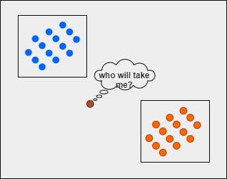
The task of putting the query point in the right class label can be tricky. We cannot just randomly assign the class label.
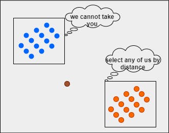
Mathematically, we have to compute the distance between the query point and each data point. We need to set a threshold and select the top nearest distance values. Let's say the threshold value is 5.
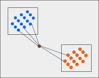
What we can see is that the query point is nearer to the blue category with 3 points and the orange category with 2 points. Now, when we apply the majority voting technique, the class label of the query point will be blue since 3 is greater than 2.
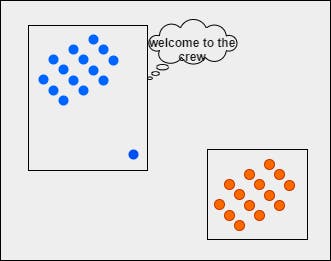
The same concept is used in developing the algorithm. Now that we have understood the theory, let's implement this totally from scratch.
Distance Measurements - Theory
Well, to compute the distance between two points, we have various methods. Here, we will just select a few distance measurement metrics.
Types of distance metrics
- Euclidean Distance
- Manhattan Distance
- Minkowski Distance
- Hamming Distance
- Cosine Distance
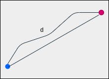
1. Euclidean Distance
The length of a line segment between any two points in the coordinate system is Euclidean distance. This metric computes the shortest distance between two points. This is also referred to as the L2 norm.
Mathematical formula
Let
$$p = [x_1, y_1]$$
and
$$q = [x_2, y_2]$$
the distance between p and q can be represented as -
$$pq = \sqrt{(x_1 - x_2)^2 + (y_1 - y_2)^2}$$
The same pattern is followed in the case of higher-dimensional vectors.
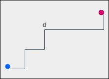
2. Manhattan Distance
Manhattan distance follows the concept of Taxicab Geometry. The usual Euclidean distance metric is replaced in such a way that the distance between points is actually the sum of absolute differences between the points. This is also referred to as the L1 norm.
Mathematical formula
Let
$$p = [x_1, y_1]$$
and
$$q = [x_2, y_2]$$
the distance between p and q can be represented as -
$$pq = |x_1 - x_2| + |y_1 - y_2|$$
The same pattern is followed in the case of higher-dimensional vectors.
3. Minkowski Distance
Minkowski distance is the generalized form of both Euclidean and Manhattan distance metrics. This is also called the Lp norm. If the value of p is 1 then it is known as Manhattan, if p is 2 then Euclidean, and so on.
Mathematical formula
Let
$$r = [x_1, y_1]$$
and
$$q = [x_2, y_2]$$
the distance between r and q can be represented as -
$$rq = \sqrt[p]{(x_1 - x_2)^p + (y_1 - y_2)^p}$$
The same pattern is followed in the case of higher-dimensional vectors.
4. Hamming Distance
The hamming distance metric is highly recommended when we are dealing with binary vectors. In case, if it is used in non-binary vectors, it produces terrible results. It is the number of bit positions in which two bits are different provided the length of two vectors are the same.
Mathematical formula
Let
$$p = [0, 1, 1, 0, 1, 0, 0]$$
and
$$q = [1, 0, 1, 0, 1, 0, 1]$$
the distance between p and q can be represented as -
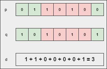
the sum of non-identical bits between the two points or vectors.
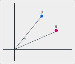
5. Cosine Distance
In order to find the angular distance, first, we have to find the cosine similarity. The similarity between two non-zero points by their inner product is called cosine similarity.
Mathematical formula
Let
$$p = [x_1, y_1]$$
and
$$q = [x_2, y_2]$$
the cosine similarity between p and q can be represented as -
$$\text{cosine-sim}(p, q) = \frac{p.q}{||p||_2 \ ||q||_2} = \frac{p.q}{\sqrt{p.p} \ \sqrt{q.q}}$$
and cosine distance between p and q can be represented as -
$$\text{cosine-dist}(p, q) = 1 - \text{cosine-sim}(p, q)$$
The same pattern is followed in the case of higher-dimensional vectors.
Distance Measurements - Code
Coding the above distance measures or metrics becomes very easy with the help of NumPy being the amazing package for numerical computation and linear algebra. Once we install it in the system, we can easily use it by importing the package.
Full code
import numpy as np

class DistanceMeasures():
    def __init__(self, point1, point2):
        """
        :param array point1: Point
        :param array point2: Point
        """
        self.point1 = np.array(point1)
        self.point2 = np.array(point2)

    def euclidean_measure(self):
        flag = True if (len(self.point1) == len(self.point2)) else False
        if flag:
            dist = np.linalg.norm(self.point1 - self.point2)
            return round(dist, 4)
        return None

    def manhattan_measure(self):
        flag = True if (len(self.point1) == len(self.point2)) else False
        if flag:
            dist = np.abs(self.point1 - self.point2).sum()
            return round(dist, 4)
        return None

    def minkowski_measure(self, p):
        flag = True if (len(self.point1) == len(self.point2)) else False

        if not flag and (p <= 0):
            return None
        if (p == 1):
            return self.manhattan_measure()
        elif (p == 2):
            return self.euclidean_measure()

        dist = np.sum(np.abs(self.point1 - self.point2) ** p) ** (1 / p)
        return round(dist, 4)

    def hamming_measure(self):
        flag = True if (len(self.point1) == len(self.point2)) else False
        if flag:
            return np.sum(self.point1 != self.point2)
        return None

    def cosine_measure(self):
        flag = True if (len(self.point1) == len(self.point2)) else False
        if flag:
            nume = np.dot(a=self.point1, b=self.point2)
            denome = np.sqrt(np.dot(a=self.point1, b=self.point1)) * np.sqrt(np.dot(a=self.point2, b=self.point2))
            return 1 - (nume / denome)
        return None
Custom KNN - Code
We have already understood the intuition of how this algorithm works. Now, we just need to apply that concept in the code. Let's do that.
Note: This article doesn't cover the performance metrics or hyperparameter tuning of the model.
Libraries
import numpy as np
import pandas as pd
import plotly.graph_objects as go

from plotly.subplots import make_subplots
from sklearn.datasets import make_classification
Construction
class KNN():
The name of the classifier is KNN and it is a class where we define other methods.
__init__() Method
    def __init__(self, n_neighbors, train_df, test_df, label, metric='euclidean'):
        """
        :param int n_neighbors: Number of nearest neighbors
        :param str metric: Distance measurement metric.
        Accepts `euclidean`, `manhattan`, `minkowski`, `hamming`, and `cosine` methods
        """
        self.n_neighbors = n_neighbors
        self.available_metrics = ['euclidean', 'manhattan', 'minkowski', 'hamming', 'cosine']
        self.metric = metric if metric in self.available_metrics else 'euclidean'

        self.X_train, self.y_train = self.split_features_targets(df=train_df, label=label)
        self.X_test, self.y_test = self.split_features_targets(df=test_df, label=label)

        self.X_train = self.X_train.values
        self.y_train = self.y_train.values
        self.X_test = self.X_test.values
        self.y_test = self.y_test.values
The above method is a constructor that takes five parameters -
n_neighbors→ refers to the number of top nearest neighbors that are used to predict the class label.train_df→ refers to the subset of the data that is used to train the classifier.test_df→ refers to the subset of the data that is used to test the classifier.label→ refers to the series of data which is actually the column name of the class label.metric→ refers to the type of distance metric that is used to compute the distance between points or vectors.
split_features_targets() Method
    def split_features_targets(self, df, label):
        """
        :param DataFrame df: The main dataset
        :param str label: The column name which signifies class labels
        :return: X, y
        """
        X = df.drop(columns=[label], axis=1)
        y = df[label]
        return X, y
The above method is used to separate features and targets from the data. It takes two parameters -
df→ refers to the entire dataset that is passed for classifying.label→ refers to the series ofdfwhich is actually the column name of the class label.
most_freq() Method
    def most_freq(self, l):
        """
        :param list l: List of values (can have duplicates)
        :return: Most occurred element from l
        """
        return max(set(l), key=l.count)
The above method is used to get the most occurred elements in the given list. Basically, this method replicates the majority voting technique that predicts the class label. It takes one parameter -
l→ refers to the list of elements (class labels).
find_nearest_neighbors() Method
    def find_nearest_neighbors(self, X_new):
        """
        :param array X_new: Array/List of each feature
        :return: distance_labels - dictionary
        """
        distances = []

        for X_row in self.X_train:
            dm = DistanceMeasures(point1=X_row, point2=X_new)

            if (self.metric == 'euclidean'):
                distances.append(dm.euclidean_measure())
            elif (self.metric == 'manhattan'):
                distances.append(dm.manhattan_measure())
            elif (self.metric == 'minkowski'):
                distances.append(dm.minkowski_measure(p=3))
            elif (self.metric == 'hamming'):
                distances.append(dm.hamming_measure())
            else:
                distances.append(dm.cosine_measure())

        distance_labels = {d : l for (d, l) in zip(distances, self.y_train)}
        distance_labels = dict(
            sorted(distance_labels.items(), key=lambda x:x[0])[:self.n_neighbors]
        )
        return distance_labels
The above method is used to find the top nearest neighbors for the query point with respect to all the data points present in the training data. It takes one parameter -
X_new→ refers to the query point for which the class label is predicted.
predict() Method
    def predict(self):
        if (len(self.X_test) == 1):
            odl = self.find_nearest_neighbors(X_new=self.X_test)
            return self.most_freq(l=list(odl.values()))

        preds = []
        for test in self.X_test:
            odl = self.find_nearest_neighbors(X_new=test)
            preds.append(self.most_freq(l=list(odl.values())))
        return np.array(preds)
The above method is used to predict the class labels for the X_test data points. It takes no parameters but uses the methods like most_freq() and find_nearest_neighbors() in order to complete the task.
score() Method
    def score(self, preds, with_plot=False):
        """
        :param array preds: Predictions
        :param boolean with_plot: True/False
        :return: accuracy level
        """
        if (len(self.y_test) == len(preds)):
            if with_plot:
                self.plot_it(preds=preds)
            return sum([1 if (i == j) else 0 for (i, j) in zip(self.y_test, preds)]) / len(preds)
        return "Lengths do not match"
The above method is used to compute the level of accuracy score that determines whether a model is performing well or not. It is a fraction of the total number of correctly classified data with the total number of all the data points. Generally, the model whose accuracy level is greater than 0.80 or 80 is considered to be a good model. It takes two parameters -
preds→ refers to an array of predictions (class labels).with_plot→ refers to a boolean value from which data visualization is decided.
plot_it() Method
    def plot_it(self, preds):
        """
        :param array preds: Predictions
        :return: None
        """
        fig = make_subplots(rows=1, cols=2)

        x_ = list(self.X_train[:, 0])
        y_ = list(self.X_train[:, 1])
        c_ = list(self.y_train)
        fig.add_trace(
            go.Scatter(x=x_, y=y_, mode='markers', marker=dict(color=c_), name='Training'),
            row=1, col=1
        )

        x_ = list(self.X_test[:, 0])
        y_ = list(self.X_test[:, 1])
        c_ = list(preds)
        fig.add_trace(
            go.Scatter(x=x_, y=y_, mode='markers', marker=dict(color=c_), name='Testing'),
            row=1, col=2
        )

        title = 'Training {} Testing'.format(' '*68)
        fig.update_layout(
            title=title, height=300, width=900,
            margin=dict(l=0, b=0, t=40, r=0), showlegend=False
        )

        fig.show()
        return None
The above method is used to visualize the data. Both training and testing data are visualized separately. It takes one parameter -
preds→ refers to an array of predictions (class labels).
Full code
class KNN():
    def __init__(self, n_neighbors, train_df, test_df, label, metric='euclidean'):
        """
        :param int n_neighbors: Number of nearest neighbors
        :param str metric: Distance measurement metric.
        Accepts `euclidean`, `manhattan`, `minkowski`, `hamming`, and `cosine` methods
        """
        self.n_neighbors = n_neighbors
        self.available_metrics = ['euclidean', 'manhattan', 'minkowski', 'hamming', 'cosine']
        self.metric = metric if metric in self.available_metrics else 'euclidean'

        self.X_train, self.y_train = self.split_features_targets(df=train_df, label=label)
        self.X_test, self.y_test = self.split_features_targets(df=test_df, label=label)

        self.X_train = self.X_train.values
        self.y_train = self.y_train.values
        self.X_test = self.X_test.values
        self.y_test = self.y_test.values

    def split_features_targets(self, df, label):
        """
        :param DataFrame df: The main dataset
        :param str label: The column name which signifies class labels
        :return: X, y
        """
        X = df.drop(columns=[label], axis=1)
        y = df[label]
        return X, y

    def most_freq(self, l):
        """
        :param list l: List of values (can have duplicates)
        :return: Most occurred element from l
        """
        return max(set(l), key=l.count)

    def find_nearest_neighbors(self, X_new):
        """
        :param array X_new: Array/List of each feature
        :return: distance_labels - dictionary
        """
        distances = []

        for X_row in self.X_train:
            dm = DistanceMeasures(point1=X_row, point2=X_new)

            if (self.metric == 'euclidean'):
                distances.append(dm.euclidean_measure())
            elif (self.metric == 'manhattan'):
                distances.append(dm.manhattan_measure())
            elif (self.metric == 'minkowski'):
                distances.append(dm.minkowski_measure(p=3))
            elif (self.metric == 'hamming'):
                distances.append(dm.hamming_measure())
            else:
                distances.append(dm.cosine_measure())

        distance_labels = {d : l for (d, l) in zip(distances, self.y_train)}
        distance_labels = dict(
            sorted(distance_labels.items(), key=lambda x:x[0])[:self.n_neighbors]
        )
        return distance_labels

    def predict(self):
        if (len(self.X_test) == 1):
            odl = self.find_nearest_neighbors(X_new=self.X_test)
            return self.most_freq(l=list(odl.values()))

        preds = []
        for test in self.X_test:
            odl = self.find_nearest_neighbors(X_new=test)
            preds.append(self.most_freq(l=list(odl.values())))
        return np.array(preds)

    def score(self, preds, with_plot=False):
        """
        :param array preds: Predictions
        :param boolean with_plot: True/False
        :return: accuracy level
        """
        if (len(self.y_test) == len(preds)):
            if with_plot:
                self.plot_it(preds=preds)
            return sum([1 if (i == j) else 0 for (i, j) in zip(self.y_test, preds)]) / len(preds)
        return "Lengths do not match"

    def plot_it(self, preds):
        """
        :param array preds: Predictions
        :return: None
        """
        fig = make_subplots(rows=1, cols=2)

        x_ = list(self.X_train[:, 0])
        y_ = list(self.X_train[:, 1])
        c_ = list(self.y_train)
        fig.add_trace(
            go.Scatter(x=x_, y=y_, mode='markers', marker=dict(color=c_), name='Training'),
            row=1, col=1
        )

        x_ = list(self.X_test[:, 0])
        y_ = list(self.X_test[:, 1])
        c_ = list(preds)
        fig.add_trace(
            go.Scatter(x=x_, y=y_, mode='markers', marker=dict(color=c_), name='Testing'),
            row=1, col=2
        )

        title = 'Training {} Testing'.format(' '*68)
        fig.update_layout(
            title=title, height=300, width=900,
            margin=dict(l=0, b=0, t=40, r=0), showlegend=False
        )

        fig.show()
        return None
Custom KNN - Testing
Before testing the model, we need to first create a toy dataset and then split it into training and testing subsets.
Data Creation
X, y = make_classification(
    n_samples=300,
    n_features=2,
    n_informative=2,
    n_redundant=0,
    n_clusters_per_class=1,
    n_classes=3,
    random_state=60
)
df = pd.DataFrame(dict(col1=X[:,0], col2=X[:,1], label=y))
The first five rows of df look like -
| col1 | col2 | label |
| 0.774027 | -1.654300 | 0 |
| 0.487983 | -0.202421 | 0 |
| 0.762589 | -0.440150 | 0 |
| -1.920213 | 0.264316 | 1 |
| 0.773207 | -0.014049 | 2 |
Data splitter
def splitter(dframe, percentage=0.8, random_state=True):
    """
    :param DataFrame dframe: Pandas DataFrame
    :param float percentage: Percentage value to split the data
    :param boolean random_state: True/False
    :return: train_df, test_df
    """
    if random_state:
        dframe = dframe.sample(frac=1)

    thresh = round(len(dframe) * percentage)
    train_df = dframe.iloc[:thresh]
    test_df = dframe.iloc[thresh:]

    return train_df, test_df
The above function is used to divide the data into two parts.
train_df, test_df = splitter(dframe=df)
Object Creation
neigh = KNN(
    train_df=train_df,
    test_df=test_df,
    label='label',
    n_neighbors=5,
    metric='cosine'
)
Prediction
preds = neigh.predict()
Accuracy Score
acc = neigh.score(preds=preds, with_plot=True)
print(acc)
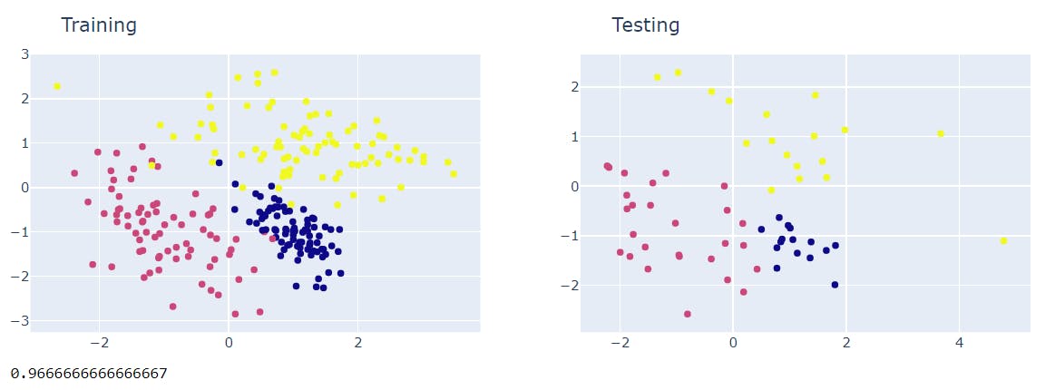
The accuracy happens to be >= 95% which is a decent percentage and hence the model is good.
Challenges
It is better to use cross-validation techniques to find the optimal value of
kto obtain better results. We did not discuss that in this article.If the data is huge, then it can very tough job for the computer as there will be time and space constraints. Because KNN happens to be slow compared to other models. Of course, we can make use of methods like
KD-TreeandLSH(Locality Sensitive Hashing) to fasten the model performance.Oftentimes, the majority voting technique may not work effectively. To avoid this problem, we can make
weighted KNNwhich works really well.It is always good to use the package methods rather than writing our own algorithms. The algorithms that we write may not be optimized enough to proceed.
References
- KNN - Wikipedia article → bit.ly/3w4cUAW
- TDS blog article → bit.ly/3x5f3ML
- Distance metrics → bit.ly/3ctuBlL
End