Introduction

In this article, we will explore the mathematics behind the image dilation operation. Like Image Erosion, Image Dilation is another important morphological operation used to increase or expand shapes contained in the input image. Think of this as “ diluting ” the image. Diluting anything requires water, here we need a structuring element or kernel.

Credits of Cover Image - Photo by Jason Leung on Unsplash

Note: We are not expanding or increasing the image size. We are increasing the pixel strength and the size remains the same.

Mathematically, we can represent this operation in the following way -

$$A \bigoplus B$$

where -

• A → Input image that is binarized
• B → structuring element or kernel

The resultant of the above formula is the dilated image. The technique that we apply here is the 2D convolution for the input image with respect to the kernel. The kernel is basically a square matrix.

Concept of Dilation

A typical binary image consists of only 1’s (255) and 0’s. The kernel can either be a subset of the input image or not which is again in the binary form. To think of this mathematically in terms of matrices — we can have:

A — the matrix of input image and B — the matrix of structuring element. The following conditions are to be applied for convolution -

1. Know the size of B to pad A by 0's. The padding width is (kernel_size - 2).
2. Position the center element of B to every element of the original input image (matrix) iteratively.
3. Extract the submatrix that is exactly equal to the size of the B.
4. Check if any (at least one) element from the submatrix is equal to the element in B considering the index location.
   • If yes, replace the element of A to 1 or 255.
   • 0, otherwise.
5. Continue this process for all the elements of A.

Note: We shall start from the first element of A till the last element of A. The GIF can be seen below to understand the convolution technique more clearly.

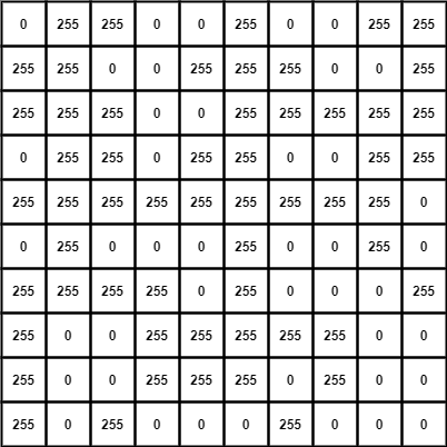
Imagine the matrix A is a binary image -

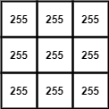
similarly, the matrix B (kernel) -

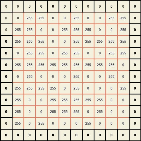
Since the kernel size is (3 x 3), we need to pad A by width (3-2) which is 1.

To extract the submatrices we can position the center element of B with every element of A and thus breaking it down, we can obtain a giant matrix where every element is a (3 x 3) submatrix of A.

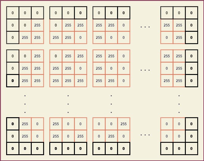
From these submatrices, we can easily map the kernel B and obtain a new value for every element of A.

The resultant image considering the input image A -

Notice the difference, we have expanded the pixels of the original image with the level of 5. The black pixels did get reduced.

Let’s code this totally from scratch using NumPy.

Time to Code

The packages that we mainly use are:

• NumPy
• Matplotlib
• OpenCV — only used for reading the image (in this article).

Import the Packages

import numpy as np
import cv2
import json
from matplotlib import pyplot as plt

Read the Image

Since we do the morphological transformations on binary images, we shall make sure whatever image we read is binarized. Therefore, we have the following functions.

def read_this(image_file):
    image_src = cv2.imread(image_file, 0)
    return image_src

def convert_binary(image_src, thresh_val):
    color_1 = 255
    color_2 = 0
    initial_conv = np.where((image_src <= thresh_val), image_src, color_1)
    final_conv = np.where((initial_conv > thresh_val), initial_conv, color_2)
    return final_conv

def binarize_this(image_file, thresh_val=127):
    image_src = read_this(image_file=image_file)
    image_b = convert_binary(image_src=image_src, thresh_val=thresh_val)
    return image_b

In the dilation function, the main parameters that are passed are:

• image_file → The input image for which the dilation operation has to be performed.

• dilation_level → In how many levels do we have to dilate the image. By default, the value of this will be 3.

• with_plot → Simply to visualize the result showing the comparison between the original image and the dilated image.

In the function —

• We obtain the kernel matrix based on the dilation_level.
• We pad the input image matrix by (kernel_size - dilation_level).
• We obtain the submatrices and replace the new values accordingly as shown in the GIF.
• Finally, we reshape the newly obtained array into the original size of the input image and plot the same.

def dilate_this(image_file, dilation_level=3, with_plot=False):
    # setting the dilation_level
    dilation_level = 3 if dilation_level < 3 else dilation_level

    # obtain the kernel by the shape of (dilation_level, dilation_level)
    structuring_kernel = np.full(shape=(dilation_level, dilation_level), fill_value=255)
    image_src = binarize_this(image_file=image_file)

    orig_shape = image_src.shape
    pad_width = dilation_level - 2

    # pad the image with pad_width
    image_pad = np.pad(array=image_src, pad_width=pad_width, mode='constant')
    pimg_shape = image_pad.shape
    h_reduce, w_reduce = (pimg_shape[0] - orig_shape[0]), (pimg_shape[1] - orig_shape[1])

    # obtain the submatrices according to the size of the kernel
    flat_submatrices = np.array([
        image_pad[i:(i + dilation_level), j:(j + dilation_level)]
        for i in range(pimg_shape[0] - h_reduce) for j in range(pimg_shape[1] - w_reduce)
    ])

    # replace the values either 255 or 0 by dilation condition
    image_dilate = np.array([255 if (i == structuring_kernel).any() else 0 for i in flat_submatrices])
    # obtain new matrix whose shape is equal to the original image size
    image_dilate = image_dilate.reshape(orig_shape)

    # plotting
    if with_plot:
        cmap_val = 'gray'
        fig, (ax1, ax2) = plt.subplots(nrows=1, ncols=2, figsize=(10, 20))

        ax1.axis("off")
        ax1.title.set_text('Original')

        ax2.axis("off")
        ax2.title.set_text("Dilated - {}".format(dilation_level))

        ax1.imshow(image_src, cmap=cmap_val)
        ax2.imshow(image_dilate, cmap=cmap_val)
        plt.show()
        return True
    return image_dilate

Now that the dilation function is ready, all that is left is testing. We will use a different image for testing.

For dilation level 3 -

dilate_this(image_file='wish.jpg', dilation_level=3, with_plot=True)

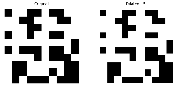
For dilation level 5 -

dilate_this(image_file='wish.jpg', dilation_level=3, with_plot=True)

In all the above results, we can notice the increase in the pixels. And this the example code developed totally from scratch. We can also rely on the cv2.dilate() method which is very faster.

References

• Morphological Transformations official documentation.