In this article, we will learn 3 ways of transposing a matrix from an easy-to-read function to an optimized code without needing any for loops.

Credits of Cover Image - Photo by Vlado Paunovic on Unsplash

Introduction

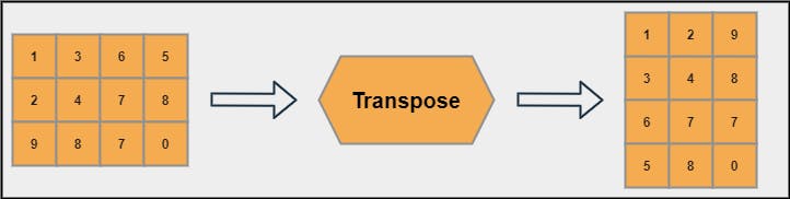
A matrix is a 2D representation of an array with M rows and N columns. An array is a collection of identical elements or objects stored in 1 row and N columns. There are so many mathematical operations and properties that can be implemented in a matrix. One such operation is the transpose operation. Transposing a matrix is easy, just converting rows into columns and vice-versa.

Let’s try to code this in 3 different ways and compare the performance.

1) Easy and Readable Function

In every matrix, the length of rows should be equal and the same follows for the columns.

We require two for loops:

• In the first loop, we consider the size of any row. This will decide the column size for our transposed matrix.

• In the second loop, we consider each row in the original matrix and extract every item order-wise.

Code

def transpose_matrix_1(matrix):
    # take the first row length
    row_len = len(matrix[0])

    trans_mat = []
    for i in range(row_len):
        trans_row = []
        for row in matrix:
            # extract every item from each row order-wise
            trans_row.append(row[i])
        trans_mat.append(trans_row)

    return trans_mat

Output

>>> matrix = [[1, 2, 3], [4, 5, 6], [7, 8, 9], [10, 11, 12]]
>>> t_matrix = transpose_matrix_1(matrix=matrix)
>>> print(t_matrix)
[[ 1  4  7 10]
 [ 2  5  8 11]
 [ 3  6  9 12]]

2) Implementing List Comprehension

We can improvise the above function by implementing list comprehension. List comprehension is easy to implement and performance-wise, it is way faster than normal for loops.

Code

def transpose_matrix_2(matrix):
    row_len = len(matrix[0])
    trans_mat = [[row[i] for row in matrix] for i in range(row_len)]
    return trans_mat

Output

>>> matrix = [[1, 2, 3], [4, 5, 6], [7, 8, 9], [10, 11, 12]]
>>> t_matrix = transpose_matrix_2(matrix=matrix)
>>> print(t_matrix)
[[ 1  4  7 10]
 [ 2  5  8 11]
 [ 3  6  9 12]]

3) Lambda Function with map() and zip()

Lambda function is a small anonymous function that takes n arguments and returns only one output.

• map() is used to map a particular function with a sequence of objects that we can achieve using for loop. But here, we don’t require any.

• zip() is used to zip every item from every row sequentially. It basically used to club things together.

Code

# zip all the items sequentially and convert it as a list
transpose_matrix_3 = lambda matrix: list(map(list, zip(*matrix)))

Output

>>> matrix = [[1, 2, 3], [4, 5, 6], [7, 8, 9], [10, 11, 12]]
>>> t_matrix = transpose_matrix_3(matrix=matrix)
>>> print(t_matrix)
[[ 1  4  7 10]
 [ 2  5  8 11]
 [ 3  6  9 12]]

Which one is Faster?

We shall compare each function’s performance based on how much time it takes to complete the task. For this, we will rely on the timeit module.

Note: We will mostly use the square matrix of different sizes. However, we can tweak the dimension values.

Code

import random
from timeit import timeit

import matplotlib.pyplot as plt
from matplotlib import style
style.use('seaborn')

def time_convertor(val, time_type):
    if time_type == 'µs':
        val = val / 1000000
    elif time_type == 'ms':
        val = val / 1000
    else:
        val = val
    return val

def compare_performace():
    r = [3, 5, 10, 50, 100, 500, 1000]
    X = []; Y1 = []; Y2 = []; Y3 = []

    for i in range(len(r)):
        matrix = [[random.randint(1, 20) for j in range(r[i])] for k in range(r[i])]

        x_val = "{} x {}".format(r[i], r[i])
        X.append(x_val)

        y_val_1 = %timeit -o transpose_matrix_1(matrix=matrix)
        y_val_2 = %timeit -o transpose_matrix_2(matrix=matrix)
        y_val_3 = %timeit -o transpose_matrix_3(matrix=matrix)
        print('---------')

        y_val_1 = str(y_val_1).split(' ', 2)
        y_val_2 = str(y_val_2).split(' ', 2)
        y_val_3 = str(y_val_3).split(' ', 2)

        y_val_1 = time_convertor(val=float(y_val_1[0]), time_type=y_val_1[1])
        y_val_2 = time_convertor(val=float(y_val_2[0]), time_type=y_val_2[1])
        y_val_3 = time_convertor(val=float(y_val_3[0]), time_type=y_val_3[1])

        Y1.append(y_val_1)
        Y2.append(y_val_2)
        Y3.append(y_val_3)

    plt.figure(figsize=(15, 8))
    plt.plot(X, Y1, '-o', label='Normal function')
    plt.plot(X, Y2, '-o', label='List comprehension')
    plt.plot(X, Y3, '-o', label='Lambda function')
    plt.xlabel('Matrix dimension')
    plt.ylabel('Function performance')
    plt.legend()
    plt.show()

    return True

2.97 µs ± 81.9 ns per loop (mean ± std. dev. of 7 runs, 100000 loops each)
2.6 µs ± 85.1 ns per loop (mean ± std. dev. of 7 runs, 100000 loops each)
1.49 µs ± 223 ns per loop (mean ± std. dev. of 7 runs, 1000000 loops each)
---------
4.65 µs ± 158 ns per loop (mean ± std. dev. of 7 runs, 100000 loops each)
4.35 µs ± 84.8 ns per loop (mean ± std. dev. of 7 runs, 100000 loops each)
1.85 µs ± 90.4 ns per loop (mean ± std. dev. of 7 runs, 1000000 loops each)
---------
13.9 µs ± 582 ns per loop (mean ± std. dev. of 7 runs, 100000 loops each)
9.82 µs ± 110 ns per loop (mean ± std. dev. of 7 runs, 100000 loops each)
3.13 µs ± 124 ns per loop (mean ± std. dev. of 7 runs, 100000 loops each)
---------
267 µs ± 10.9 µs per loop (mean ± std. dev. of 7 runs, 1000 loops each)
144 µs ± 2.41 µs per loop (mean ± std. dev. of 7 runs, 10000 loops each)
29.7 µs ± 863 ns per loop (mean ± std. dev. of 7 runs, 10000 loops each)
---------
1.02 ms ± 27.2 µs per loop (mean ± std. dev. of 7 runs, 1000 loops each)
527 µs ± 9.94 µs per loop (mean ± std. dev. of 7 runs, 1000 loops each)
113 µs ± 1.89 µs per loop (mean ± std. dev. of 7 runs, 10000 loops each)
---------
33.1 ms ± 815 µs per loop (mean ± std. dev. of 7 runs, 10 loops each)
20.9 ms ± 887 µs per loop (mean ± std. dev. of 7 runs, 10 loops each)
3.58 ms ± 57.4 µs per loop (mean ± std. dev. of 7 runs, 100 loops each)
---------
120 ms ± 1.71 ms per loop (mean ± std. dev. of 7 runs, 10 loops each)
73.1 ms ± 3.08 ms per loop (mean ± std. dev. of 7 runs, 10 loops each)
20 ms ± 1.73 ms per loop (mean ± std. dev. of 7 runs, 100 loops each)

Performance Graph

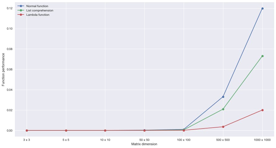
The time complexity is similar for our first and second functions — O(M*N). But when we compare, the list comprehension is always faster than a regular for loop.

In the other case, where we used the lambda function, it is quite faster than the list comprehension. All I had to do is simply use the built-in functions which are always faster than user-defined functions.