San Francisco - City

San Francisco is the cultural, commercial, and financial capital of the state of California in the United States. It is the 17th most populated city in the United States and a renowned tourist destination noted for its cool summers, the Golden Gate Bridge, and some of the world's best restaurants. Despite being a city known for its growth, San Francisco remains one of the most dangerous places to live due to an increase in criminal activities.

SF OpenData - an open data catalog of San Francisco has provided 12 years of crime data dated from 1/1/2003 to 5/13/2015. These criminal records are mostly the incidents derived from SFPD Crime Incident Reporting System. They have published this dataset on Kaggle.

The main agenda of this whole case study is to predict the category of the crime for the incident that can occur in the future. Thus, helping them reduce the time and effort of organizing the data.

ML Problem Formulation

Data Overview

1. Source → kaggle.com/c/sf-crime/data

2. In total, we have 3 files

   • train.csv.zip
   • test.csv.zip
   • sampleSubmission.csv.zip

3. The training data has 9 columns that include the target column as well.

4. The test data has 6 columns that exclude the target column (this is something we need to predict).

Problem Type

• There are 39 different classes of crimes that need to be classified.
• Hence this leads to a multi-class classification problem.

Performance Metric

Since it is a classification problem, the metrics that we stick to are -

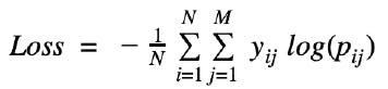
• Multi Log-Loss - the ultimate aim of any machine learning model is to reduce the loss. For this problem, a perfect classifier would be the one that reduces the multiclass logarithmic loss to 0.

• Confusion Matrix - is a summary of prediction results on a classification problem. The number of correct and incorrect predictions are summarized with count values and broken down by each class.

Objectives & Constraints

1. Predict the probability of each data point belonging to each of the 39 classes.
2. Constraints:
   • Interpretability
   • Class probabilities are needed
   • Penalize the errors in class probabilities => Metric is Log-loss
   • No latency constraints

Exploratory Data Analysis

The original training data that are given -

The original test data that are given -

Clearly, from the Dates column we can extract time-based features such as -

• date
• year
• month
• day
• hour
• minute
• season
• hour_type
• time_period

Also, from the Address column we can extract the address type such as -

Training data after extracting time-based and address-type features.

Test data after extracting time-based and address-type features.

Univariate Analysis

So, we got some important features. We can perform the univariate analysis considering each column and get to know how the data is distributed.

Target Distribution

• The above is the class distribution of the column category.
• Clearly, we can see that Larceny/Theft is the most occurred type of crime in the all the years.
• The last 5 to 6 crimes are negligible, meaning they occurred very rarely.
• The data is not balanced. Therefore, while building the model it is better to do the stratification-based splitting.

Address-type Distribution

• From the above plot, we can tell that most of the crimes occurred on Streets and Crosses.
  • St stands for the street.
  • Cross signifies the junction point.

Police-department Distribution

• Southern is the bay area where most of the crimes got reported.

Year Distribution

• We know that the data is recorded from 1/1/2003 to 5/13/2015.
  • The data of the year 2015 is not recorded fully.
• The year 2013 has more number crimes. Others also have a similar occurrence range.

Month Distribution

• In all of the months, we can observe that the occurrence of the crimes roughly ranges from 60k to 80k.

Weekday (Day) Distribution

• Friday is the day where most of the crimes occurred.
• Sunday is the day when fewer crimes (compared with other days) occurred.
  • This is more likely because it is a holiday.
• This distribution is almost similar.

Hour Distribution

• It is observed from the above that most of the crimes happen either in the evening or at midnight.

Time-period Distribution

• We can observe that most of the crimes usually happen either during the evening or at night.

Hour-type Distribution

• Morning, Mid-Night, and Night are considered to be the time period suitable for crimes to be happening.
  • In fact, they have a similar distribution.
• Evening and Noon are the time periods where the business is usually continuous.

Occurrences Yearly

• The above is an animation plot showing the occurrences that had happened yearly.
• The above is the count of each occurrence type that occurred in the police department.
• The most common crime that occurred is Larceny/Theft.
• This is something we observed in the plot of overall occurrences in all the years.

Map Visualization Yearly

• The above shows the exact location of the types of crimes that occurred per police department.
• This is a year-wise plot and the police department that is chosen is Richmond.

Choropleth Visualization Monthly

• The above is the choropleth map based on the count of the occurrences per police department.
• Southern is the police department where most of the crimes got reported.
• This is a month-wise plot for the year 2015.

Geo-Density Map

• The GIF showcases the density map of the top 12 crimes that occurred per year.
• The most important thing to observe in this is that Larency/Theft is always present at first.
  • The second is Other Offenses.
• The density is taken in descending order and hence retains the top crimes.

Multivariate Analysis

In order to do multivariate analysis, we must require other features based on the columns that we have. We can follow the below steps to obtain them.

1. Categorical columns can be encoded to One-Hot-Encoding.
   • Procedure to follow up - here.
2. We can extract the spatial distance features by considering all the police stations in San Francisco and computing the haversine distance between each station to all the coordinate values that are present in the data.
   • Procedure to follow up - here.
3. We can perform some arithmetic operations between latitude and longitude. These are known as location-based features.
   • Procedure to follow up - here.
4. Address column can be converted to Bog of Words and TF-IDF representations.
   • Procedure to follow up - here.
5. In doing so, we end up with 130 features. This is pretty good to learn from the data. Earlier we had around 7 features.

We shall visualize a TSNE plot to see whether we can separate the classes fully or not. Since the data is large, I have considered only the 10% of the whole data by performing a stratification split. The reason for doing this is because TSNE consumes more time to get trained. The 10% of the whole data is almost 87804 data points.

TSNE - 10%

• Currently, the dataset consists of 39 classes.
• From the above plot, we can clearly see that the data is highly imbalanced.
• The clusters are not separated properly.

TSNE - 10% (top 12 crimes)

• The above is better compared to when we considered all the categories.
• The clusters also formed in a better way.
• The separation of the clusters is also better.

TSNE - 10% (top 5 crimes)

• The above plot is far better compared to all the previous plots.
• We can see the separation clearly.

Modeling & Training

Now that we got the features it is time for us to apply various classification models and check the performance of each. For this problem, we will go with the following models.

• Logistic Regression
• Decision Tree
• Random Forest
• XGBoost Classifier

We can also try

• KNN

I did not implement it as it consumes more time to train and due to the system's inefficiency, I opted to skip it.

Let's train some models...

Dummy Classifier

Also known as a random model. This model assigns a random class label for each data point. This is helpful in order to check if other important models do better than this or not. The loss that we obtain from this - can be set as a threshold and thus aiming to achieve the minimum loss than the threshold.

Logistic Regression

After hyperparameter tuning, it happens the best value of C to be 30 and l2 as a regulariser. We proceed with log loss since accuracy won't help as the data is imbalanced. Fortunately, the loss is lesser than the loss of the dummy classifier.

When the model is tested on the test data, the overall Kaggle score is -

Decision Tree

After hyperparameter tuning, it happens the best value of max_depth to be 50 and min_samples_split to be 500. We proceed with log loss since accuracy won't help as the data is imbalanced. Fortunately, the loss is lesser than the loss of the dummy classifier.

When the model is tested on the test data, the overall Kaggle score is -

Random Forest

After hyperparameter tuning, it happens the best value of max_depth to be 8 and n_estimators to be 100. We proceed with log loss since accuracy won't help as the data is imbalanced. Fortunately, the loss is lesser than the loss of the dummy classifier.

When the model is tested on the test data, the overall Kaggle score is -

XGBoost Classifier

After hyperparameter tuning, it happens the best value of max_depth to be 8 and n_estimators to be 150. We proceed with log loss since accuracy won't help as the data is imbalanced. Fortunately, the loss is lesser than the loss of the dummy classifier.

When the model is tested on the test data, the overall Kaggle score is -

We have to calibrate the probabilities (predictions), as probability is playing a vital role in the problem of classifying.

The results of StackingClassifier are not up to the mark.

Models' Summary

• From the above, we can observe that all models (except DummyClassifier) performed well.
  • The loss of each model is less than the DummyClassifier.
  • The best model compared to all other models is XGBoost. The loss of this very little.

The full code for modeling can be found here.

Single Point Prediction

As part of this, we need to predict the category of the crime when the original test data (single point) is passed as input to the model. This is important in real-life scenarios as we do not generally pass the features and preprocessed test data to the model.

The code for the single-point prediction can be found here.

The video demonstration.

Jovian Project Link -

LinkedIn Profile -

References

1. appliedaicourse.com

2. towardsdatascience.com/why-training-set-sho..

3. towardsdatascience.com/leveraging-geolocati..

4. slideshare.net/RohitDandona/san-francisco-c..

5. researchgate.net/publication/305288147_San_..

6. cseweb.ucsd.edu/classes/wi15/cse255-a/repor..

Future Work

We can attempt to apply deep learning-based models and check the performance with respect to the already trained models that we did. To my knowledge, most of the kagglers who attempted to solve this problem implemented their solutions using deep learning models. We can definitely give it a try.