Linear Regression Algorithm in Practice

Introduction

Regression analysis is a process of predicting a response variable given an explanatory variable. The response variable is also called a dependent variable and an explanatory variable is known as an independent variable. Given a problem statement, when there are multiple explanatory variables and one response variable, then the process is known as Multiple Linear Regression. On contrary, if a problem statement contains only one explanatory variable and one response variable, it is known as Simple Linear Regression.

Note - For implementing regression analysis, there needs to be a strong relationship between the explanatory variable and the response variable.

Unlike predicting the class label (in classification task), here we predict the real value (continuous value) for the new unseen data.

Credits of Cover Image - Photo by Stary Smok on Unsplash

Mathematical Model

Let's denote the response variable as y and the explanatory variable as X. Here X, can take either a single feature or multiple features.

In the case of X having one feature, the model would be -

$$\hat{y} = w^Tx + b \rightarrow (1)$$

In the case of X having multiple features, the model would be -

$$X = [x_1, x_2, x_3, \dots, x_n]$$

$$\hat{y} = w_1x_1 + w_2x_2 + w_3x_3 + \dots + w_nx_n + b$$

$$\hat{y} = \sum_{i=1}^n w_ix_i + b$$

$$\hat{y} = W^TX + b \rightarrow (2)$$

The mathematical model (1) is used for simple linear regression tasks, whereas (2) for multiple linear regression tasks. In both cases, the response variable y^ is the target feature.

The actual response variable is denoted as y and we all know that the machine learning model cannot predict very accurately. If it cannot predict accurately, it surely contains an error. Thus, the main focus now shifted to have errors as small as possible.

$$y = \hat{y} + E \rightarrow (3)$$

Substituting (1) in (3) for simple linear regression, we get -

$$y = w^Tx + b + E \rightarrow (4)$$

Substituting (2) in (3) for multiple linear regression, we get -

$$y = W^TX + b + E \rightarrow (5)$$

The error E is the difference between the actual target feature and the predicted target feature.

$$E = (y - \hat{y})$$

Everything is properly written except two things which are still unknown. The two things are the parameters w and b. The error in the model depends on these two parameter values. Here, w is the coefficient and b is the intercept. We cannot simply assign random values for w and b. Instead, they are to be chosen wisely with the help of the stochastic gradient descent process.

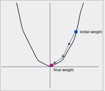
Stochastic Gradient Descent (SGD)

Let's consider the model equation (1) for understanding optimization.

SGD is an iterative process where we initially assign random values (possibly 0) for both w and b. At every iteration,

For w, we differentiate (1) with respect to w and obtain dw.
For b, we differentiate (1) with respect to b and obtain db.

Mathematically, it can be represented as -

$$dw \implies \frac{\partial}{\partial w} = \frac{2}{N} \sum_{i=1}^n x_i \big[(w^Tx_i + b) - y_i \big]$$

and

$$db \implies \frac{\partial}{\partial b} = \frac{2}{N} \sum_{i=1}^n \big[(w^Tx_i + b) - y_i \big]$$

We update/replace the actual w and b with dw and db respectively at every iteration until the values are not fully minimized. The updating process can be understood in the following way.

$$w = w - \alpha * dw$$

and

$$b = b - \alpha * db$$

The entire process is the same for obtaining the minimal values of W and b for the model equation (2).

Now that we have understood the complete process, let's implement the same from scratch.

Linear Regression - Code

We will start by importing the necessary libraries as always at the start.

Libraries

import warnings
warnings.filterwarnings('ignore')

import os
import pandas as pd
import numpy as np
import imageio

from matplotlib import pyplot as plt
from sklearn.datasets import make_regression

Data Creation

For now, we will depend on a toy dataset that we can easily create by the module sklearn.

X, y = make_regression(n_samples=200, n_features=1, noise=5, random_state=15)
df = pd.DataFrame(dict(col1=X[:, 0], col2=y))

Data Splitter

We need to split the data into two - the training set and the testing set. We do this by a random splitter function.

def splitter(dframe, percentage=0.8, random_state=True):
    """
    :param DataFrame dframe: Pandas DataFrame
    :param float percentage: Percentage value to split the data
    :param boolean random_state: True/False
    :return: train_df, test_df
    """
    if random_state:
        dframe = dframe.sample(frac=1)

    thresh = round(len(dframe) * percentage)
    train_df = dframe.iloc[:thresh]
    test_df = dframe.iloc[thresh:]

    return train_df, test_df

Train Test Split

train_df, test_df = splitter(dframe=df)

Construction

class LinearRegression():

The name of the regression is LinearRegression and it is a class where we define other methods.

`init()` Method

    def __init__(self, train_df, test_df, label, lambda_=0.001, n_iters=1000):
        self.n_iters = n_iters
        self.lambda_ = lambda_

        self.X_train, self.y_train = self.split_features_targets(df=train_df, label=label)
        self.X_test, self.y_test = self.split_features_targets(df=test_df, label=label)
        self.X_train = self.X_train.values
        self.y_train = self.y_train.values
        self.X_test = self.X_test.values
        self.y_test = self.y_test.values

        self.n_train = len(self.X_train)
        self.n_test = len(self.X_test)
        self.wb_params = {'w' : [], 'b' : []}
        self.w, self.b = self.find_best_params()

The above method is a constructor that takes five parameters -

train_df → refers to the subset of the data that is used to train the regressor.
test_df → refers to the subset of the data that is used to test the regressor.
label → refers to the series of data which is actually the column name of the class label.
lambda_ → refers to a constant that is used to update the parameters during the process of SGD.
n_iters → refers to a constant that is used to decide the total iterations of the process of SGD.

`split_features_targets()` Method

    def split_features_targets(self, df, label):
        X = df.drop(columns=[label], axis=1)
        y = df[label]
        return X, y

The above method is used to separate features and targets from the data. It takes two parameters -

df → refers to the entire dataset that is passed for classifying.
label → refers to the series of df which is actually the column name of the class label.

`diff_params_wb()` Method

    def diff_params_wb(self, w, b):
        lm = np.dot(self.X_train, w) + b
        w_ = (2 / self.n_train) * np.dot(self.X_train.T, (lm - self.y_train))
        b_ = (2 / self.n_train) * np.sum((lm - self.y_train))
        return w_, b_

The above method is used to differentiate the parameters. It takes two parameters -

w → refers to the initial weight vector that is used in the process of SGD.
b → refers to the initial intercept value that is used in the process of SGD.

`find_best_params()` Method

    def find_best_params(self):
        ow = np.zeros_like(a=self.X_train[0])
        ob = 0

        for i in range(self.n_iters):
            w_, b_ = self.diff_params_wb(w=ow, b=ob)
            ow = ow - (self.lambda_ * w_)
            ob = ob - (self.lambda_ * b_)
            self.wb_params['w'].append(ow)
            self.wb_params['b'].append(ob)

        return ow, ob

The above method is used to get the best (minimal) values of the parameters w and b. It takes no functional parameters. This method follows the process of SGD to update the original values of w and b iteratively.

`predict()` Method

   def predict(self, with_plot=False, save_process=False):
        y_test_preds = np.dot(self.X_test, self.w) + self.b
        y_train_preds = np.dot(self.X_train, self.w) + self.b

        if with_plot:
            fig = plt.figure(figsize=(10, 4))

            ax1 = fig.add_subplot(1, 2, 1)
            ax1.title.set_text('Training')
            ax1.scatter(self.X_train, self.y_train, label='points')
            ax1.plot(self.X_train, y_train_preds, color='red', label='best fit')
            ax1.legend()

            ax2 = fig.add_subplot(1, 2, 2)
            ax2.title.set_text("Testing")
            ax2.scatter(self.X_test, self.y_test, label='points')
            ax2.plot(self.X_test, y_test_preds, color='red', label='best fit')
            ax2.legend()

            plt.show()

        if save_process:
            self.save_process_togif(test_x=self.X_test, test_y=self.y_test)

        return y_test_preds

The above method is used to predict the real (continuous) value for the new unseen data. It takes two parameters (which are optional) -

with_plot → refers to a boolean value to decide if to plot the best fit line along with the data points.
save_process → refers to a boolean value to decide if to save the process of SGD in GIF format.

By default, these functional parameters take the False value and therefore optional.

`save_process_togif()` Method

    def save_process_togif(self, test_x, test_y):
        wp = self.wb_params['w']
        bp = self.wb_params['b']

        c = 0
        for i in range(0, len(wp), 50):
            c += 1
            d = '0' + str(c) if (len(str(c)) == 1) else str(c)
            test_p = np.dot(test_x, wp[i]) + bp[i]

            fig = plt.figure(figsize=(10, 10))
            plt.title("Testing")
            plt.scatter(test_x, test_y, label='points')
            plt.plot(test_x, test_p, color='red', label='best fit')
            plt.legend()
            plt.savefig('{}-lr-plot.png'.format(d))
            plt.close(fig)

        path = os.getcwd()
        files_list = os.listdir(path=path)
        png_list = [i for i in files_list if (i[0] != '.') and (i.split('.')[1] == 'png')]
        png_list.sort()
        png_gif = [imageio.imread(i) for i in png_list]
        kargs = {'duration': 1}
        gif_name = 'process-lin-reg.gif'
        imageio.mimsave(gif_name, png_gif, **kargs)
        print('Process saved in → ', path + '\\' + gif_name)

        return None

The above method is used to save the process of SGD in the form of GIF. It takes two parameters -

test_x → refers to the features whose target needs to be predicted.
test_y → refers to the actual target values.

`score()` Method

    def score(self, preds):
        preds = np.array(preds)

        if (len(self.y_test) == len(preds)):
            y_act_mean = np.mean(self.y_test)
            sst = np.sum((self.y_test - y_act_mean) ** 2)
            ssr = np.sum((self.y_test - preds) ** 2)
            return (1 - (ssr / sst))
        return "Lengths do not match"

The above method is used to calculate the R^2. It takes one parameter -

preds → refers to the predicted values that are used to calculate R^2.

Full Code

class LinearRegression():
    def __init__(self, train_df, test_df, label, lambda_=0.001, n_iters=1000):
        self.n_iters = n_iters
        self.lambda_ = lambda_

        self.X_train, self.y_train = self.split_features_targets(df=train_df, label=label)
        self.X_test, self.y_test = self.split_features_targets(df=test_df, label=label)
        self.X_train = self.X_train.values
        self.y_train = self.y_train.values
        self.X_test = self.X_test.values
        self.y_test = self.y_test.values

        self.n_train = len(self.X_train)
        self.n_test = len(self.X_test)
        self.wb_params = {'w' : [], 'b' : []}
        self.w, self.b = self.find_best_params()

    def split_features_targets(self, df, label):
        X = df.drop(columns=[label], axis=1)
        y = df[label]
        return X, y

    def diff_params_wb(self, w, b):
        lm = np.dot(self.X_train, w) + b
        w_ = (2 / self.n_train) * np.dot(self.X_train.T, (lm - self.y_train))
        b_ = (2 / self.n_train) * np.sum((lm - self.y_train))
        return w_, b_

    def find_best_params(self):
        ow = np.zeros_like(a=self.X_train[0])
        ob = 0

        for i in range(self.n_iters):
            w_, b_ = self.diff_params_wb(w=ow, b=ob)
            ow = ow - (self.lambda_ * w_)
            ob = ob - (self.lambda_ * b_)
            self.wb_params['w'].append(ow)
            self.wb_params['b'].append(ob)

        return ow, ob

    def predict(self, with_plot=False, save_process=False):
        y_test_preds = np.dot(self.X_test, self.w) + self.b
        y_train_preds = np.dot(self.X_train, self.w) + self.b

        if with_plot:
            fig = plt.figure(figsize=(10, 4))

            ax1 = fig.add_subplot(1, 2, 1)
            ax1.title.set_text('Training')
            ax1.scatter(self.X_train, self.y_train, label='points')
            ax1.plot(self.X_train, y_train_preds, color='red', label='best fit')
            ax1.legend()

            ax2 = fig.add_subplot(1, 2, 2)
            ax2.title.set_text("Testing")
            ax2.scatter(self.X_test, self.y_test, label='points')
            ax2.plot(self.X_test, y_test_preds, color='red', label='best fit')
            ax2.legend()

            plt.show()

        if save_process:
            self.save_process_togif(test_x=self.X_test, test_y=self.y_test)

        return y_test_preds

    def save_process_togif(self, test_x, test_y):
        wp = self.wb_params['w']
        bp = self.wb_params['b']

        c = 0
        for i in range(0, len(wp), 50):
            c += 1
            d = '0' + str(c) if (len(str(c)) == 1) else str(c)
            test_p = np.dot(test_x, wp[i]) + bp[i]

            fig = plt.figure(figsize=(10, 10))
            plt.title("Testing")
            plt.scatter(test_x, test_y, label='points')
            plt.plot(test_x, test_p, color='red', label='best fit')
            plt.legend()
            plt.savefig('{}-lr-plot.png'.format(d))
            plt.close(fig)

        path = os.getcwd()
        files_list = os.listdir(path=path)
        png_list = [i for i in files_list if (i[0] != '.') and (i.split('.')[1] == 'png')]
        png_list.sort()
        png_gif = [imageio.imread(i) for i in png_list]
        kargs = {'duration': 1}
        gif_name = 'process-lin-reg.gif'
        imageio.mimsave(gif_name, png_gif, **kargs)
        print('Process saved in → ', path + '\\' + gif_name)

        return None

    def score(self, preds):
        preds = np.array(preds)

        if (len(self.y_test) == len(preds)):
            y_act_mean = np.mean(self.y_test)
            sst = np.sum((self.y_test - y_act_mean) ** 2)
            ssr = np.sum((self.y_test - preds) ** 2)
            return (1 - (ssr / sst))
        return "Lengths do not match"

Linear Regression - Testing

We have already created a toy data set. We just need to test the model on that data.

Note: The data that we created is random. Results may differ for each execution.

Object Creation

lr = LinearRegression(
    train_df=train_df, 
    test_df=test_df, 
    label='col2', 
    lambda_=0.01, 
    n_iters=1000
)

Weights

print(lr.w)
# [5.90699167]

Intercept

print(lr.b)
# -0.5282539569012746

Prediction

preds = lr.predict(with_plot=True, save_process=True)

Training & Testing Plot

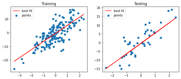
The regression line sufficiently passes through the data points.

SGD Process Demonstration

The test values are used to execute the process of SGD. As the values of w and b change for every iteration the best fit line changes accordingly, and at some point, the line stops changing, which basically means that we have got the minimum values for w and b.

Performance Score

print(lr.score(preds=preds))
# 0.6830871781610702

The accuracy is almost 69% for the data whose shape is (200, 2). If we had taken/created large data, then there would have been some change.

Challenges

Well, this entire code is been developed from scratch and it is sure that it, by performance - may not be as efficient as the library methods. But, it was good to understand the mathematics behind the work.

My code is slow.
No regularization is implemented although there types of it.
- Linear regression with L1 regularization is known as Ridge regression.
- Linear regression with L2 regularization is known as Lasso regression.
- Linear regression with both L1 and L2 regularizations is known as ElasticNet regression.
If outliers are present in the data, it may impact the model significantly.

References

YouTube video → bit.ly/2TRmnxd
Wikipedia article → en.wikipedia.org/wiki/Linear_regression

End

Linear Regression Algorithm in Practice

What the linear regression algorithm is and how it is used in regression tasks.

Table of contents

Introduction

Mathematical Model

Stochastic Gradient Descent (SGD)

Linear Regression - Code

Libraries

Data Creation

Data Splitter

Construction

`init()` Method

`split_features_targets()` Method

`diff_params_wb()` Method

`find_best_params()` Method

`predict()` Method

`save_process_togif()` Method

`score()` Method

Linear Regression - Testing

Object Creation

Weights

Intercept

Prediction

Performance Score

Challenges

References

Linear Regression Algorithm in Practice

What the linear regression algorithm is and how it is used in regression tasks.

Table of contents

Introduction

Mathematical Model

Stochastic Gradient Descent (SGD)

Linear Regression - Code

Libraries

Data Creation

Data Splitter

Construction

__init__() Method

split_features_targets() Method

diff_params_wb() Method

find_best_params() Method

predict() Method

save_process_togif() Method

score() Method

Linear Regression - Testing

Object Creation

Weights

Intercept

Prediction

Performance Score

Challenges

References

`init()` Method

`split_features_targets()` Method

`diff_params_wb()` Method

`find_best_params()` Method

`predict()` Method

`save_process_togif()` Method

`score()` Method