Complete Understanding of Morphological Transformations in Image Processing

Introduction

In this article, we will explore other transformations where image erosion and image dilation stand as a base. In the previous articles on morphological transformations, we learned the two important transformations namely erosion and dilation.

The transformations that are built on top of these two are -

• Opening
• Closing
• Morphological Gradient
• Top hat
• Black hat
• Boundary Extraction
• Hit — Miss Transformation

We have seen a step-by-step implementation of erosion and dilation explaining the convolution method with simple matrix operations. In all of these transformations, we rely on the binary input image and a structuring element or kernel. The structuring element needs to be a square matrix which is again a binary matrix.

Note: If you are not familiar with erosion and dilation. I would recommend you refer to my previous articles.

• Image Erosion → bit.ly/3gcojco
• Image Dilation → bit.ly/2TlOncd

For now, we will consider

• A → input image matrix
• B → kernel matrix

Credits of Cover Image - Photo by Suzanne D. Williams on Unsplash

Opening Transformation / Image Opening

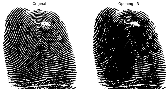
We know erosion and dilation are quite opposite to each other. But Opening is just another name of erosion followed by dilation. Mathematically, we can represent it as -

$$(A \circ B) \rightarrow (1)$$

If we further break it down, we can represent it as -

$$(A \circ B) = (A \ominus B) \oplus B \rightarrow (2)$$

Eq (1) is represented in terms of erosion and dilation, the same can be seen in Eq (2).

This transformation is helpful in removing the noise from the image.

Closing Transformation / Image Closing

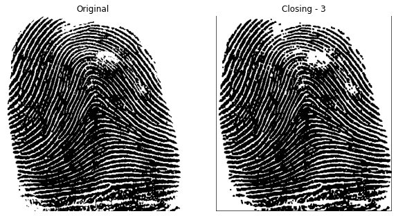
Closing transformation is quite opposite of Opening transformation. Closing is just another name of a dilation followed by erosion. Mathematically, we can represent it as -

$$(A \bullet B) \rightarrow (3)$$

If we further break it down, we can represent it as -

$$(A \bullet B) = (A \oplus B) \ominus B \rightarrow (4)$$

Eq (3) is represented in terms of dilation and erosion, the same can be seen in Eq (4).

This transformation is helpful in closing the holes in the foreground object of the image.

Morphological Gradient

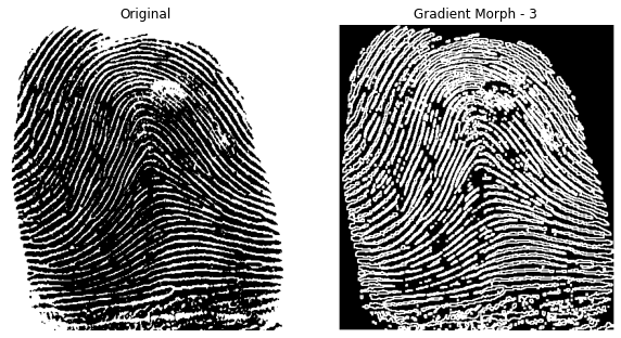
The morphological gradient can be easily obtained once we have the eroded image and dilated image. It is the difference between dilated image and an eroded image. Mathematically, we can represent it as -

$$(A \oplus B) - (A \ominus B)$$

The resultant of this transformation appears to be an outline of the foreground object.

Top Hat Transformation

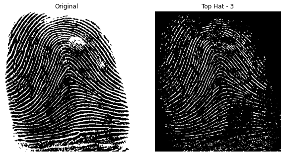
Top Hat transformation is the difference between the input image and the opening of the image. Mathematically, we can represent it as -

$$A - (A \circ B) \rightarrow (5)$$

If we further break it down, we can represent it as -

$$A - [\ (A \ominus B) \oplus B \ ] \rightarrow (6)$$

Eq (5) is represented in terms of erosion and dilation, the same can be seen in Eq (6).

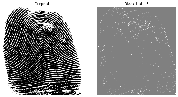
Black Hat Transformation

Back Hat transformation is the difference between the closing of the input image and the input image. Mathematically, we can represent it as -

$$(A \bullet B) - A \rightarrow (7)$$

If we further break it down, we can represent it as -

$$[\ (A \oplus B) \ominus B \ ] - A \rightarrow (8)$$

Eq (7) is represented in terms of dilation and erosion, the same can be seen in Eq (8).

Boundary Extraction

Boundary extraction is one of the applications of morphological transformations. In simple words, it is the difference between the input image and the eroded image. Mathematically, we can represent it as -

$$A - (A \ominus B)$$

The boundary of the foreground object is represented in white color and the rest be in black color. If we do the reverse process, i.e., the difference between the input image and dilated image — the boundary will get in black color, and the rest will be in white color.

---

Time to Code

The packages that we mainly use are:

• NumPy
• Matplotlib
• OpenCV

import the Packages

import numpy as np
import cv2
import json
from matplotlib import pyplot as plt

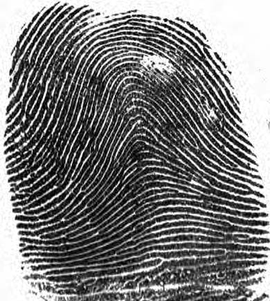
For the entire implementation, I will be using the finger-print image, you can use the same for the practice.

Code — Morphological Transformations

class MorphologicalTransformations(object):
    def __init__(self, image_file, level):
        self.level = 3 if level < 3 else level
        self.image_file = image_file
        self.MAX_PIXEL = 255
        self.MIN_PIXEL = 0
        self.MID_PIXEL = self.MAX_PIXEL // 2
        self.kernel = np.full(shape=(level, level), fill_value=255)

    def read_this(self):
        image_src = cv2.imread(self.image_file, 0)
        return image_src

    def convert_binary(self, image_src, thresh_val):
        color_1 = self.MAX_PIXEL
        color_2 = self.MIN_PIXEL
        initial_conv = np.where((image_src <= thresh_val), image_src, color_1)
        final_conv = np.where((initial_conv > thresh_val), initial_conv, color_2)
        return final_conv

    def binarize_this(self):
        image_src = self.read_this()
        image_b = self.convert_binary(image_src=image_src, thresh_val=self.MID_PIXEL)
        return image_b

    def get_flat_submatrices(self, image_src, h_reduce, w_reduce):
        image_shape = image_src.shape
        flat_submats = np.array([
            image_src[i:(i + self.level), j:(j + self.level)]
            for i in range(image_shape[0] - h_reduce) for j in range(image_shape[1] - w_reduce)
        ])
        return flat_submats

    def erode_image(self, image_src, with_plot=False):
        orig_shape = image_src.shape
        pad_width = self.level - 2

        image_pad = np.pad(array=image_src, pad_width=pad_width, mode='constant')
        pimg_shape = image_pad.shape

        h_reduce, w_reduce = (pimg_shape[0] - orig_shape[0]), (pimg_shape[1] - orig_shape[1])
        flat_submats = self.get_flat_submatrices(
            image_src=image_pad, h_reduce=h_reduce, w_reduce=w_reduce
        )

        image_eroded = np.array([255 if (i == self.kernel).all() else 0 for i in flat_submats])
        image_eroded = image_eroded.reshape(orig_shape)

        if with_plot:
            self.plot_it(orig_matrix=image_src, trans_matrix=image_eroded, head_text='Eroded - {}'.format(self.level))
            return None
        return image_eroded

    def dilate_image(self, image_src, with_plot=False):        
        orig_shape = image_src.shape
        pad_width = self.level - 2

        image_pad = np.pad(array=image_src, pad_width=pad_width, mode='constant')
        pimg_shape = image_pad.shape

        h_reduce, w_reduce = (pimg_shape[0] - orig_shape[0]), (pimg_shape[1] - orig_shape[1])
        flat_submats = self.get_flat_submatrices(
            image_src=image_pad, h_reduce=h_reduce, w_reduce=w_reduce
        )

        image_dilated = np.array([255 if (i == self.kernel).any() else 0 for i in flat_submats])
        image_dilated = image_dilated.reshape(orig_shape)

        if with_plot:
            self.plot_it(orig_matrix=image_src, trans_matrix=image_dilated, head_text='Dilated - {}'.format(self.level))
            return None
        return image_dilated

    def open_image(self, image_src, with_plot=False):
        image_eroded = self.erode_image(image_src=image_src)
        image_opening = self.dilate_image(image_src=image_eroded)

        if with_plot:
            self.plot_it(orig_matrix=image_src, trans_matrix=image_opening, head_text='Opening - {}'.format(self.level))
            return None
        return image_opening

    def close_image(self, image_src, with_plot=False):
        image_dilated = self.dilate_image(image_src=image_src)
        image_closing = self.erode_image(image_src=image_dilated)

        if with_plot:
            self.plot_it(orig_matrix=image_src, trans_matrix=image_closing, head_text='Closing - {}'.format(self.level))
            return None
        return image_closing

    def morph_gradient(self, image_src, with_plot=False):
        image_dilated = self.dilate_image(image_src=image_src)
        image_eroded = self.erode_image(image_src=image_src)
        image_grad = image_dilated - image_eroded

        if with_plot:
            self.plot_it(orig_matrix=image_src, trans_matrix=image_grad, head_text='Gradient Morph - {}'.format(self.level))
            return None
        return image_grad

    def extract_boundary(self, image_src, with_plot=False):
        image_eroded = self.erode_image(image_src=image_src)
        ext_bound = image_src - image_eroded

        if with_plot:
            self.plot_it(orig_matrix=image_src, trans_matrix=ext_bound, head_text='Boundary - {}'.format(self.level))
            return None
        return ext_bound

    def get_tophat(self, image_src, with_plot=False):
        image_opening = self.open_image(image_src=image_src)
        image_tophat = image_src - image_opening

        if with_plot:
            self.plot_it(orig_matrix=image_src, trans_matrix=image_tophat, head_text='Top Hat - {}'.format(self.level))
            return None
        return image_tophat

    def get_blackhat(self, image_src, with_plot=False):
        image_closing = self.close_image(image_src=image_src)
        image_blackhat = image_closing - image_src

        if with_plot:
            self.plot_it(orig_matrix=image_src, trans_matrix=image_blackhat, head_text='Black Hat - {}'.format(self.level))
            return None
        return image_blackhat

    def plot_it(self, orig_matrix, trans_matrix, head_text):
        fig, (ax1, ax2) = plt.subplots(nrows=1, ncols=2, figsize=(10, 20))
        cmap_val = 'gray'

        ax1.axis("off")
        ax1.title.set_text('Original')

        ax2.axis("off")
        ax2.title.set_text(head_text)

        ax1.imshow(orig_matrix, cmap=cmap_val)
        ax2.imshow(trans_matrix, cmap=cmap_val)
        plt.show()
        return True

Object Creation

morph = MorphologicalTransformations(
    image_file='Finger-arch.jpg', 
    level=3
)
image_src = morph.binarize_this()

In the above code, we have made an object called morph, and using this object we are converting the input image into a binary image.

Erosion

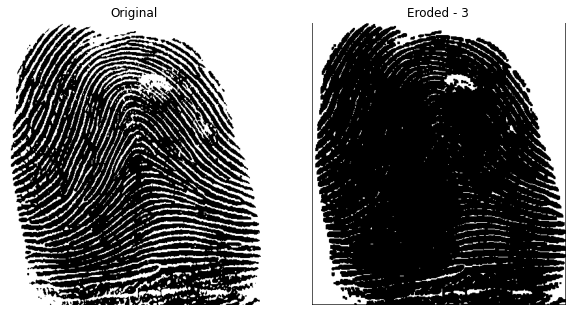
morph.erode_image(image_src=image_src, with_plot=True)

Dilation

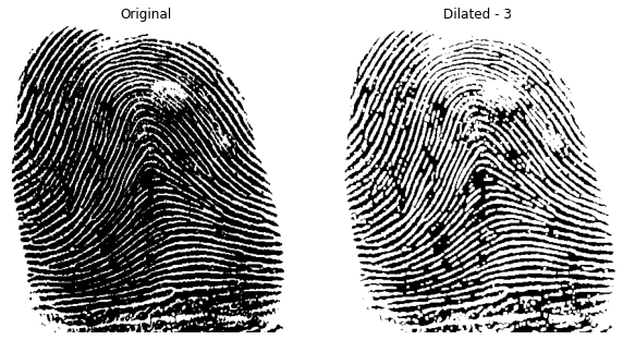
morph.dilate_image(image_src=image_src, with_plot=True)

Opening

morph.open_image(image_src=image_src, with_plot=True)

Closing

morph.close_image(image_src=image_src, with_plot=True)

Morphological Gradient

morph.morph_gradient(image_src=image_src, with_plot=True)

Top Hat

morph.get_tophat(image_src=image_src, with_plot=True)

Black Hat

morph.get_blackhat(image_src=image_src, with_plot=True)

Boundary Extraction

morph.extract_boundary(image_src=image_src, with_plot=True)

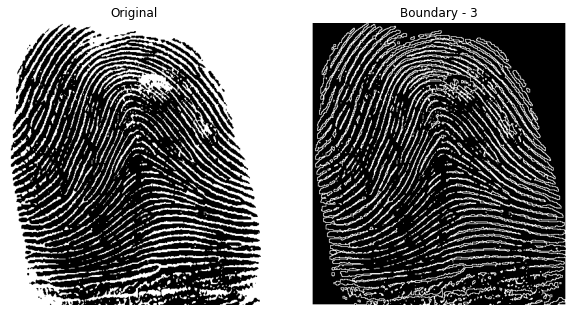
These are the results of all the transformations. We obtained these with the help of erosion and dilation.

Note: All of the code is written from scratch using the NumPy library.

---

Conclusion

In this article, we have almost covered the types of morphological transformations. Although, there are some advanced transformations like Hit — Miss Transformation, which I didn’t cover in this but definitely next time.

When we have speed and compatibility constraints, I would recommend using the official library methods. This was just practiced to understand the inner working and mathematics behind each algorithm.

End