#7 - Handle Missing Values in Data
Strategies to handle missing values


What is a missing value?
Missing value simply refers to a situation where there is no data stored for the variable in an observation. This usually happens when there is no response detected for a particular question during the process of data collection. Data Analysts have to be very careful in dealing with missing values. The process to handle the missing data is called imputation. On the whole, imputation is helpful to some extent but not fully in replacing the actual value that can be assumed in the place of missing value.
Credits of Cover Image - Photo by Alex Jones on Unsplash
Techniques of Imputation
- Filling by a Central Tendency
- Mean replacement
- Median replacement
- Mode replacement
- Categorical Imputation
- For each category, compute central tendency and fill the missing value for that category itself.
- Model Imputation
- Building a machine learning model to fill up the missing data by the predicted values.
Note - In this article, we will focus only on 1 and 2 techniques. We will not focus on 3 just for now.
For implementing the above methods we will need to first create a toy dataset in order to programmatically understand each technique.
Necessary imports
import warnings
warnings.filterwarnings('ignore')

import pandas as pd
import numpy as np
import random

from sklearn.datasets import make_blobs
from scipy import stats
from matplotlib import pyplot as plt
Dataset Creation
In our data, we shall make sure that we have at least one feature which is categorical. The method make_blobs() can be really handy in creating toy datasets in our own experiments.
With this method, we will create a dataset that will have -
- 100 samples
- 2 features
- 3 centers
X, y = make_blobs(n_samples=100, n_features=2, centers=3)
df = pd.DataFrame(dict(x=X[:,0], y=X[:,1], label=y))
print(df.head())
The gist of the data looks like this -
| Index | x | y | label |
| 0 | -1.960223 | -2.240400 | 2 |
| 1 | -3.489893 | -3.149356 | 2 |
| 2 | -8.173217 | 6.186763 | 1 |
| 3 | -1.216968 | -3.318524 | 2 |
| 4 | -7.661975 | 9.092514 | 1 |
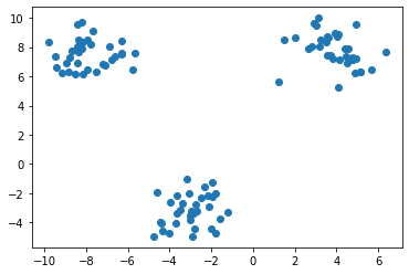
Similarly, the original plot of the data looks like this -
Missing values at random locations
In Python, a missing value is represented as NaN which means Not a Number. We will create missing values in the y column for the above toy dataset.
df['y'].loc[df['y'].sample(frac=0.1).index] = np.nan
The above code simply means that we are creating 10% of missing values completely at random locations of the existing data frame.
df.isnull().sum()

# ------
'''
x         0
y        10
label     0
dtype: int64
'''
Computing Central Tendency
Since, we have to impute the missing values with central tendencies like mean, median, and mode. We will create a helper function that takes three params -
data→ The dataset for which the central tendencies should be computed.col→ The column for which the central tendencies should be computed.strategy→ Mean, Median, and Mode strategies.
def fill_values(data, col, strategy):
    if (strategy == 'mean'):
        fval = data[col].mean()
    elif (strategy == 'median'):
        fval = data[col].mean()
    else:
        fval = stats.mode(data[col])[0][0]
    return fval
The above function returns a value based on the strategy that is used.
1) Filling by a Central Tendency
In order to fill the NaN values with new values in the existing column of the data, we need to have a function that does so. The function takes three params -
data→ The dataset for which the central tendencies should be computed.col→ The column for which the central tendencies should be computed.strategy→ Mean, Median, and Mode strategies.
def simple_imputer(data, col, strategy):
    fval = fill_values(data=data, col=col, strategy=strategy)
    non_nans = data[col].fillna(fval).to_list()
    return non_nans
The above function returns a list with filled values based on the strategy that is used.
Note - The above technique is very simple and would not produce good results when compared with other techniques.
If we try to visualize the data after filling the NaN's, we would see some sort of dispersion in the data.
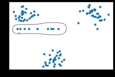
We can see a horizontal pattern formed by points. These points are actually NaN values that got filled by a respective central tendency. And moreover, neither of them belong to any of the clusters.
2) Categorical Imputation
In our original dataset, besides x and y columns we also have one column called label that 3 unique values such as [0, 1, 2]. A simple hack that we can incorporate here is, we can separate the data by clusters and then compute the central tendency to fill up the NaN values. By doing so, we can make sure that the new values belong to their respective clusters.
As usual, we will have a function to separate data cluster-wise. The function takes four params -
data→ The dataset for which the central tendencies should be computed.col→ The column for which the central tendencies should be computed.label→ The column with which the data is separated into clusters.strategy→ Mean, Median, and Mode strategies.
def label_imputer(self, data, col, label, strategy):
    col_label_df = data[[col, label]]
    counts_df = col_label_df[label].value_counts().to_frame()
    classes = counts_df.index.to_list()

    fval_class = []
    for each_class in classes:
        # separating data into clusters
        mini_frame = col_label_df[col_label_df[label] == each_class]
        # computing central tendency
        non_nans_frame = pd.Series(data=simple_imputer(mini_frame, col, strategy), index=mini_frame.index)
        fval_class.append(non_nans_frame)
    final_vals = pd.concat(fval_class).sort_index().to_list()

    return final_vals
The above function is used to compute the central tendency value based upon the cluster that it belongs to and finally returns a list of values.
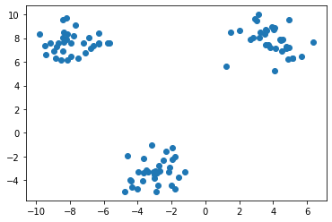
If we try to visualize the data after filling the NaN's, we would not see any sort of dispersion in the data but rather a uniformity and resemblance with the original plot (without NaN values).
Full Code
class Imputer():
    def __init__(self, strategy):
        self.available_strats = ['mean', 'median', 'mode']
        self.strategy = 'median' if strategy not in self.available_strats else strategy

    def fill_values(self, data, col):
        if (self.strategy == 'mean'):
            fval = data[col].mean()
        elif (self.strategy == 'median'):
            fval = data[col].mean()
        else:
            fval = stats.mode(data[col])[0][0]
        return fval

    def simple_imputer(self, data, col):
        fval = self.fill_values(data=data, col=col)
        non_nans = data[col].fillna(fval).to_list()
        return non_nans

    def label_imputer(self, data, col, label):
        col_label_df = data[[col, label]]
        counts_df = col_label_df[label].value_counts().to_frame()
        classes = counts_df.index.to_list()

        fval_class = []
        for each_class in classes:
            mini_frame = col_label_df[col_label_df[label] == each_class]
            non_nans_frame = pd.Series(data=self.simple_imputer(data=mini_frame, col=col), index=mini_frame.index)
            fval_class.append(non_nans_frame)
        final_vals = pd.concat(fval_class).sort_index().to_list()

        return final_vals
Conclusion
Throughout this article, we saw different techniques to handle the missing data. But, this was implemented on a toy dataset, not on a real dataset.
Practicing the above on real data may or may not be suitable. And moreover, it is quite impossible to have a categorical feature to separate the data in clusters and fill the values based on the clusters themselves.
It might be beneficial to practice the third technique which predicts the missing values by a mathematical model and this is an unbiased technique that entirely depends on the training data and a model itself.
It is all up to the practitioner to choose any method and come up with a solution for the given problem.
Buy Me Coffee
If you have liked my article you can buy some coffee and support me here. That would motivate me to write and learn more about what I know.
Well, that's all for now. This article is included in the series Exploratory Data Analysis, where I share tips and tutorials helpful to get started. We will learn step-by-step how to explore and analyze the data. As a pre-condition, knowing the fundamentals of programming would be helpful. The link to this series can be found here.