Introduction

Identifying or selecting the important features is one of the crucial processes in data science and data analytics. After all, the features that are selected decide how qualitative the data is. It is exactly like the phrase Garbage in, Garbage out - meaning, whatever features that we consider, the result of the whole analytical process depends on those features. It is also said that data analysts spend at least 60 to 70 percent of their time preparing the data.

Credits of Cover Image - Photo by Brian Lundquist on Unsplash

What is Data Preprocessing?

Data Preprocessing is an important phase of the whole analytical process, where relevant fields are extracted or queried from the gathered data. It is in this step, data analysts try their best to retain or increase the quality of the data, with which further steps become handy. During the process of data gathering, it is quite sure to end up collecting messy data and therefore it has to be preprocessed right after it is collected. It includes steps like -

• Data Cleaning - In this process, unnecessary data values which do not add importance are removed. Mostly, it includes missing values that should be cleaned or filled.

• Data Editing - In this process, the original data is edited or changed in order to maintain uniqueness. For example, in the dataset, if there is an age column then it is important to have all the age values in numeric, and there can be chances to get the data in non-numeric. In that case, it is always encouraged to edit the data.

• Data Wrangling - In this process, the raw data is transformed or manipulated in such a format that it is easy to use and readily available for data analytics. Oftentimes, it is also called data manipulation.

Note - The above steps are explained in a nutshell. Moreover, the overall complexity (to maintain data quality) depends on the dataset that is collected.

Importance of Correlation

Correlation is a statistical measurement that tells how one feature is affecting the target variable. It returns a percentage value describing the relationship. The correlation value (percentage) lies between -1 and +1.

• -1 → describes that the feature and the target variables are negatively correlated, meaning - one increases when the other decreases and vice-versa.

• 0 → describes that there is no correlation.

• +1 → describes that the feature and the target variables are positively correlated, meaning - one increases when the other increases and vice-versa.

Correlation is really helpful in knowing those features that actually affect the target variable.

Let's try to identify which features are important in one dataset.

Note - Throughout this series, we will be dealing with one dataset originally taken from Kaggle.

Hands-on Practice

For the hands-on practice, we will use a dataset in the domain of health care on heart attack possibility.

Let's get started ...

We are using Python and specifically Pandas library - developed with a clear intention to approach the key aspects of data analytics and data science problems.

Installation

pip install pandas --user
pip install numpy --user
pip install seaborn --user
pip install matplotlib --user

The above installs the current version of packages in the system. Let's import the same.

import pandas as pd
import numpy as np
import seaborn as sns

from matplotlib import pyplot as plt

Load / Read

In order to load or read the data, we use the read_csv() method where we explicitly tell Pandas that we want to read a CSV file.

df = pd.read_csv('heart.csv)

Since df is a Pandas object, we can instantiate the other methods that are made available to understand the data.

Display the 1st Five Rows

df.head()

head() is used to display the first five rows. By default, we don't explicitly mention how many we want to display. However, if you want to display other than five rows you can mention a number like head(<any_number>).

  age sex cp trestbps chol fbs restecg thalach exang oldpeak slope ca  thal target
0 63  1   3  145      233  1   0       150     0     2.3     0     0   1    1
1 37  1   2  130      250  0   1       187     0     3.5     0     0   2    1
2 41  0   1  130      204  0   0       172     0     1.4     2     0   2    1
3 56  1   1  120      236  0   1       178     0     0.8     2     0   2    1
4 57  0   0  120      354  0   1       163     1     0.6     2     0   2    1

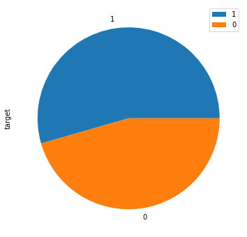
We have a column called target that has two unique values.

• 0 → indicates fewer chances of getting a heart attack
• 1 → indicates more chances of getting a heart attack

Count the data by target column

To count the frequency of the data we will use the value_counts() method.

ha_df = df['target'].value_counts().to_frame()

The above methods convert the count (data) to a data frame.

    target
----------
1   165
0   138

Visually, we can represent the above count (data) as a pie chart.

ha_df.plot(kind='pie', figsize=(10, 6), subplots=True)
plt.show()

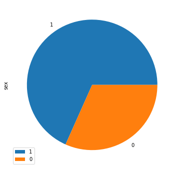
Count the data by sex ratio

From the original data frame df, we have a column called sex which is again numerical where -

• 1 → indicates male
• 0 → indicates female

Let's visualize the pie chart of the same.

sdf = df['sex'].value_counts().to_frame()
sdf.plot(kind='pie', figsize=(10, 6), subplots=True)
plt.show()

Identify Important Features with Correlation Plot

With the help of Pandas, we can easily find correlations considering the entire data frame.

cor_df = df.corr()

This will return the correlations to each column with all the other columns. We can directly visualize the correlation matrix using seaborn plots.

plt.figure(figsize=(10, 6))

sns.heatmap(
    data=cor_df,
    vmin=-1,
    vmax=1,
    center=0,
    cmap='seismic',
    annot=True
)

plt.show()

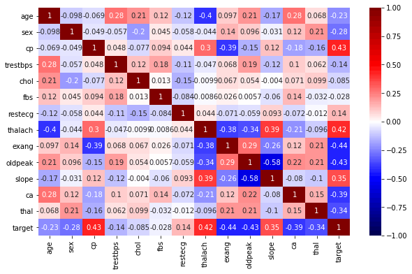
If we carefully observe the correlation matrix, there are totally 3 features that are affecting the target variable. They are -

• cp - chest pain
• thalach - heartbeat rate
• slope - may be

The variable chol (cholesterol) has no relationship. In fact, from the correlation plot, we see that the relationship ratio is -0.085. Whereas, cp and thalach have around 0.43 and 0.42 respectively.

---

Well, that's all for now. This article is included in the series Exploratory Data Analysis, where I share tips and tutorials helpful to get started. We will learn step-by-step how to explore and analyze the data. As a pre-condition, knowing the fundamentals of programming would be helpful. The link to this series can be found here.