Introduction

If you had read my previous articles on matrix operations, by now you would have already know what a matrix is. Yes, a matrix is a 2D representation of an array with M rows and N columns. The shape of the matrix is generally referred to as dimension. Thus the shape of any typical matrix is represented or assumed to have (M x N) dimensions.

Credits of Cover Image - Photo by Carl Nenzen Loven on Unsplash

• Row Matrix - Collection of identical elements or objects stored in 1 row and N columns.

• Column Matrix - Collection of identical elements or objects stored in N rows and 1 column.

Note - Matrices of shapes (1 x N) and (N x 1) are generally called row vector and column vector respectively.

Algorithm Explanation

For instance, let's assume we have two matrices A and B. The general rule before multiplying is that the number of COLUMNS of A should be exactly equal to the number of ROWS of B. If this rule is satisfied then -

We shall compute the dot product for each row of A with respect to each column of B. This process continues until there are no elements left to compute.

• Each row of A is considered to be a row vector.
• Each column of B is considered to be a column vector.
• Dot Product - It is an algebraic operation that is computed on two equal-sized vectors which result in a single number. It is also called a scalar product. Mathematically, we represent it in the form of -

$$r.c = \sum_{i=1}^{n} r_i c_i \rightarrow \text{for} \ i = \text{1 to n}$$

The resultant matrix's (after operation) size would be equal to the number of ROWS of A and the number of COLUMNS of B.

Note - The computation can be risky or slow when we are dealing with large matrices. This can be easily handled by NumPy.

GIF Explanation

GIF by Author

Easy to read function

If we try to break down the whole algorithm, the very first thing that we have to do is to transpose one of the matrices and compute the dot or scalar product for each row of the matrix to each column of the other matrix.

Matrix Transpose

def transpose(m):
    trans_mat = [[row[i] for row in m] for i in range(len(m[0]))]
    return trans_mat

Dot Product

def scalar_product(r, c):
    ps = [i * j for (i, j) in zip(r, c)]
    return sum(ps)

Matrix Multiplication

def mats_product(m1, m2):
    m2_t = transpose(m=m2)
    mats_p = [[scalar_product(r=r, c=c) for c in m2_t] for r in m1]
    return mats_p

To wrap all the functions together, we can do the following -

Wrap Up

def easy_product(m1, m2):    
    def transpose(m):
        trans_mat = [[row[i] for row in m] for i in range(len(m[0]))]
        return trans_mat

    def scalar_product(r, c):
        ps = [i * j for (i, j) in zip(r, c)]
        return sum(ps)

    def mats_product(m1, m2):
        m2_t = transpose(m=m2)
        mats_p = [[scalar_product(r=r, c=c) for c in m2_t] for r in m1]
        return mats_p

    return mats_product(m1, m2)

More simplified code - (Optimized)

The above easy_product() can still be optimized by using the built-in methods of Python. Better improvement is needed on the method transpose().

Matrix Transpose

transpose = lambda m : list(map(list, zip(*m)))

Dot Product

The above scalar_product() can still be reduced and maintained like -

scalar_product = lambda r, c: sum([i * j for (i, j) in zip(r, c)])

Matrix Multiplication

def mats_product(m1, m2):
    m2_t = transpose(m=m2)
    mats_p = [[scalar_product(r=r, c=c) for c in m2_t] for r in m1]
    return mats_p

To wrap all the functions together, we can do the following -

Wrap Up

def optimized_product(m1, m2):
    transpose = lambda m : list(map(list, zip(*m)))
    scalar_product = lambda r, c: sum([i * j for (i, j) in zip(r, c)])

    def mats_product(m1, m2):
        m2_t = transpose(m=m2)
        mats_p = [[scalar_product(r=r, c=c) for c in m2_t] for r in m1]
        return mats_p

    return mats_product(m1, m2)

Awesome! Both the functions are ready to be tested. In order to test so, we need to have matrices defined. We will create random matrices (function) which can further be helpful to check the speed compatibility of both functions.

Random matrices creation

import random

def create_matrix(rcount, ccount):
    random.seed(10)
    m = [[random.randint(10, 80) for i in range(ccount)] for j in range(rcount)]
    return m

Testing Phase

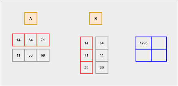
>>> nr = 2
>>> nc = 3
>>> 
>>> m1 = create_matrix(nr, nc)
>>> m2 = create_matrix(nc, nr)
>>> m1
[[14, 64, 71], [11, 36, 69]]
>>> m2
[[14, 64], [71, 11], [36, 69]]

Normal Function

>>> mm = easy_product(m1, m2)
>>> print(mm)
[[7296, 6499], [5194, 5861]]

Improved Code

>>> mm = optimized_product(m1, m2)
>>> print(mm)
[[7296, 6499], [5194, 5861]]

Speed and Computation - Comparison

Now, both the functions seem working well enough. But it is also important to check the algorithm performance in terms of speedy computation and time.

For this, we will run both the functions in a loop for a defined set of matrix shapes and store the required amount of time that each takes. We shall also plot the same to represent it visually.

Performance Check

import time
from matplotlib import pyplot as plt

def check_speed():
    shapes = [(3, 2), (5, 4), (10, 9), (20, 5), (30, 8), (40, 2), (50, 10), (2, 10), (5, 80), (100, 34), (200, 100), (300, 200)]

    x = [str(i) for i in shapes]
    y1 = []; y2 = [];

    for sp in shapes:
        m1 = create_matrix(sp[0], sp[1])
        m2 = create_matrix(sp[1], sp[0])

        start_e = time.time()
        res_easy = easy_product(m1, m2)
        end_e = time.time()
        easy_elapse = end_e - start_e

        start_o = time.time()
        res_opt = optimized_product(m1, m2)
        end_o = time.time()
        opt_elapse = end_o - start_o

        y1.append(easy_elapse)
        y2.append(opt_elapse)

    plt.figure(figsize=(15, 6))
    plt.plot(x, y1, 'o-', label='Normal Function')
    plt.plot(x, y2, 'o-', label='Optimized Code')
    plt.legend()
    plt.show()

    return None

Performance Graph

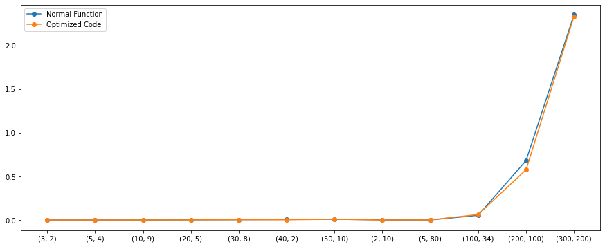
Both the algorithms seem to work similarly except for few cases. But there is a catch, we wrote these functions from a personal point. If we introduce NumPy for doing the same, the performance would be much better. The below graph includes the performance of NumPy as well.

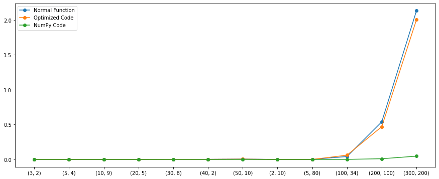
Yes! NumPy is much faster. NumPy consumes very little time to compute the same operation no matter what the sizes are.

Things I Learnt

• Breaking down a given problem and approaching each one to ultimately solve the original problem.

• Comparing algorithms and tracking the computation.

---

Buy Me Coffee

If you have liked my article you can buy some coffee and support me here. That would motivate me to write and learn more about what I know.