Introduction

The main agenda of this article to analyze crime data by following all the steps required for the complete data analysis. The steps include Data Preparation, Data Cleaning, Data Wrangling, Feature Selection, Data Visualization & Comparison.

The data is about the crimes committed against women in India. The data is being recorded from 2001 to 2014. It includes crimes like -

• Rape
• Kidnapping and Abduction
• Dowry Deaths
• Assault on Women with intent to outrage her modesty
• Insult to the modesty of Women
• Cruelty by Husband or his Relatives
• Importation of Girls

Data Source → Crimes Against Women - kaggle.com

Throughout this article, we will try to see if at all there is a reduction in crimes as the year count increases. We will visualize each column of data (mentioned above) state-wise & year-wise, and thus explore in a much better way. If you want to directly check out my work at Kaggle, feel free to visit this notebook.

Credits of Cover Image - Photo by Stefano Pollio on Unsplash

Libraries

As always, begin with importing all the necessary packages.

import warnings
warnings.filterwarnings('ignore')

import requests
import pandas as pd
import numpy as np
import plotly.graph_objects as go

Data Reading

I have saved the CSV data in my local system with the file name caw_2001-2014.csv.

df = pd.read_csv('caw_2001-2014.csv', index_col=0)

Data Preparation

• We will rename all the columns ensuring that the column name is short and precise for easy access to the column.

df.columns = ['state_unit', 'district', 'year', 'rape', 'kidnap_abduction', 'dowry_deaths', 
              'women_assault', 'women_insult', 'husband_relative_cruelty', 'girl_importation']
df.index = list(range(df.shape[0]))

• There is a lot of string data where all the values are uppercased. To maintain uniqueness and flexibility, we will convert all the string values to title-case.

for col in df.columns:
    df[col] = df[col].apply(lambda x : x.title() if isinstance(x, str) else x)

• If we observe the column - state_unit, there are few values that need replacement. Some values are repetitive, in the sense that it signifies the same meaning but has a different name. We shall replace all those values to have a single unique name. This process is really helpful in order to visualize the data geographically.

replacements = {
    'A & N Islands' : 'Andaman and Nicobar',
    'A&N Islands' : 'Andaman and Nicobar',
    'Daman & Diu' : 'Daman and Diu',
    'Delhi Ut' : 'Delhi',
    'D & N Haveli' : 'Dadra and Nagar Haveli',
    'D&N Haveli' : 'Dadra and Nagar Haveli',
    'Odisha' : 'Orissa',
    'Jammu & Kashmir' : 'Jammu and Kashmir'
}

for (o, r) in replacements.items():
    df['state_unit'].replace(to_replace=o, value=r, inplace=True)

Data Exploration & Categorization

• Since the data is being collected from 2001 till 2014. We will need to split the data year-wise and save it in a dictionary. This is simply an efficient way of organizing the data.

def split_data(dframe):
    min_year = dframe['year'].min()
    max_year = dframe['year'].max()

    data_year_wise = {
        year : dframe[dframe['year'] == year] for year in range(min_year, max_year + 1)
    }

    return data_year_wise

# --------------

data_splits = split_data(dframe=df)

• To know the dimension of the data (year-wise), we can iterate through each key and print the shape of each value.

for (y, d) in data_splits.items():
    print(y, '\t→', d.shape)

# --------------
'''
2001     → (716, 10)
2002     → (719, 10)
2003     → (728, 10)
2004     → (729, 10)
...
2014     → (837, 10)
'''

• In the column district, there is one unique row that has the total number of crime counts pertaining to each column. This again differs based on the name of the state_unit.

def categorize_crimes(data_source, state_unit=None):
    crime_list = list(data_source[2001].columns[3:])

    all_crimes_year_wise = {}
    for (y, d) in data_source.items():
        y_df = d[d['district'].str.contains('Total')]
        if state_unit:
            y_df = y_df[y_df['state_unit'] == state_unit.title()]
        crime_dict = {col : y_df[col].sum() for col in crime_list}
        # all_crimes_year_wise[y] = dict(sorted(crime_dict.items(), key=lambda x:x[1], reverse=True))
        all_crimes_year_wise[y] = crime_dict

    return all_crimes_year_wise

The above function categorize_crimes() takes two parameters such as -

• data_source → refers to the entire data which is split based on year.
• state_unit → refers to the name of the state or unit. If the value is None, it considers total crime counts year-wise on the basis of the whole country. Otherwise, it considers total crime counts year-wise on the basis of a particular state.

Now that we have organized data categorized, we can visualize it to identify the patterns.

Data Visualization & Analysis

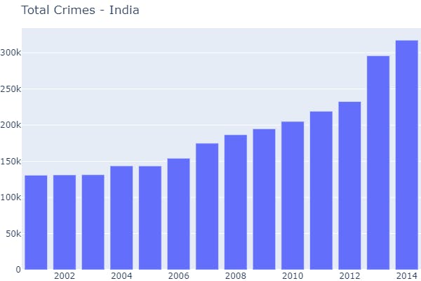
Visualizing the count of crimes considering the whole country by including all the crimes.

1. For this, we will create a function that takes the total number of crimes either state-wise or country-wise. We just need to provide the data_source and state_unit is optional.

2. Once it obtains the total count of each column, again sums up all the columns to get the whole total of crimes that happened every year.

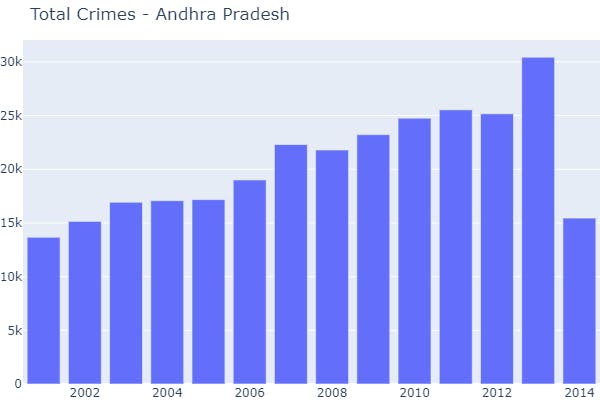
3. If state_unit is specified, it does the same process but only limited to that particular state.

def plot_overall_crimes_by_year(data_source, state_unit=None, kind='bar'):
    crimes_data = categorize_crimes(data_source=data_source, state_unit=state_unit)
    year_sum_crimes = {y : sum(list(cr.values())) for (y, cr) in crimes_data.items()}

    y_keys = list(year_sum_crimes.keys())
    y_vals = list(year_sum_crimes.values())

    t = 'Total Crimes - {}'
    title = t.format(state_unit.title()) if state_unit else t.format('India')

    if kind == 'bar':
        trace = go.Bar(x=y_keys, y=y_vals)
    else:
        trace = go.Pie(labels=y_keys, values=y_vals)

    layout = go.Layout(
        height=400,
        width=600,
        title=title,
        margin=dict(l=0, r=0, b=0, t=40)
    )

    fig = go.Figure(data=[trace], layout=layout)
    fig.show()

    return None

• 1 Function Call → Visualization on the basis of the whole country.

plot_overall_crimes_by_year(data_source=data_splits)

• 2 Function Call → Visualization on the basis of a particular state.

plot_overall_crimes_by_year(data_source=data_splits, state_unit='Andhra Pradesh')

---

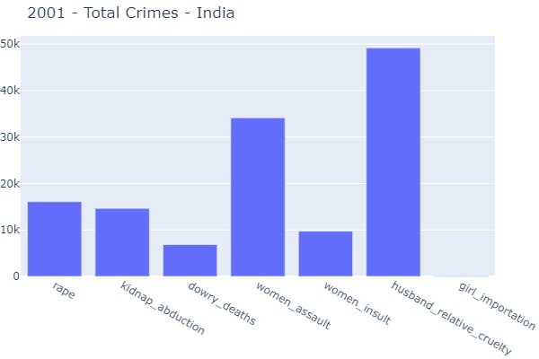
Visualizing the count of crimes considering the whole country by including all the crimes and a specific year in which they took place.

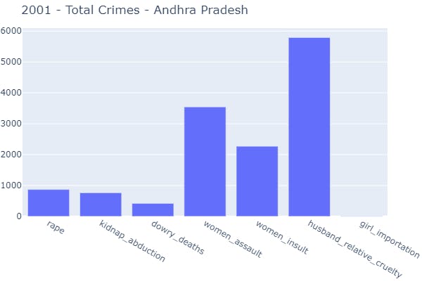
1. For this, we will create a function that takes the total number of crimes either state-wise or country-wise by year. We just need to provide the data_source, year, and state_unit is optional.

2. If state_unit is specified, it does the same process but only limited to that particular state.

def plot_crimes_by_year(data_source, year, state_unit=None, kind='bar'):
    crimes_data = categorize_crimes(data_source=data_source, state_unit=state_unit)
    year_all_crimes = crimes_data[year]

    y_keys = list(year_all_crimes.keys())
    y_vals = list(year_all_crimes.values())

    t = '{} - Total Crimes - {}'
    title = t.format(year, state_unit.title()) if state_unit else t.format(year, 'India')

    if kind == 'bar':
        trace = go.Bar(x=y_keys,y=y_vals)
    else:
        trace = go.Pie(labels=y_keys, values=y_vals)

    layout = go.Layout(
        height=400,
        width=600,
        title=title,
        margin=dict(l=0, r=0, b=0, t=40)
    )

    fig = go.Figure(data=[trace], layout=layout)
    fig.show()

    return None

• 1 Function Call → Visualization on the basis of the whole country in a specific period of time (year).

plot_crimes_by_year(data_source=data_splits, year=2001)

• 2 Function Call → Visualization on the basis of a particular state in a specific period of time (year).

plot_crimes_by_year(data_source=data_splits, year=2001, state_unit='Andhra Pradesh')

---

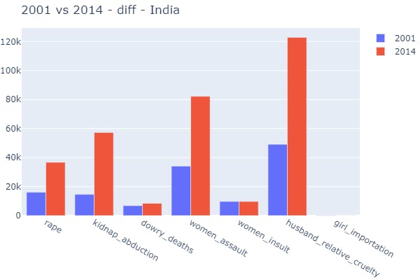
Comparing the difference of occurrences visually by both country-wise and a particular state-wise considering two different periods of time (years).

1. For this, we will create a function that takes the total number of crimes either state-wise or country-wise by two different years. We just need to provide the data_source, ideal_year, cwith_year, and state_unit is optional.

2. If state_unit is specified, it does the same process but only limited to that particular state.

def plot_overall_difference(data_source, ideal_year, cwith_year, state_unit=None):
    crime_data = categorize_crimes(data_source=data_source, state_unit=state_unit)

    ideal_year_crimes = crime_data[ideal_year]
    cwith_year_crimes = crime_data[cwith_year]

    t = '{} vs {} - diff - {}'
    title = t.format(ideal_year, cwith_year, state_unit.title()) if state_unit else t.format(ideal_year, cwith_year, 'India')

    trace1 = go.Bar(
        x=list(ideal_year_crimes.keys()),
        y=list(ideal_year_crimes.values()),
        name=ideal_year
    )
    trace2 = go.Bar(
        x=list(cwith_year_crimes.keys()),
        y=list(cwith_year_crimes.values()),
        name=cwith_year
    )

    layout = go.Layout(
        height=400,
        width=600,
        title=title,
        margin=dict(l=0, r=0, b=0, t=40)
    )

    fig = go.Figure(data=[trace1, trace2], layout=layout)
    fig.show()

    return None

• 1 Function Call → Visualization on the basis of the whole country in two different periods of time (years).

plot_overall_difference(data_source=data_splits, ideal_year=2001, cwith_year=2014)

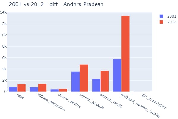
• 2 Function Call → Visualization on the basis of a particular state in two different periods of time (years).

plot_overall_difference(data_source=data_splits, ideal_year=2001, cwith_year=2012, state_unit='Andhra Pradesh')

---

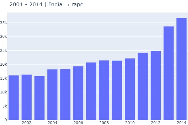
Plotting a particular crime both country-wise and state-wise to identify increasing or decreasing patterns yearly-wise.

1. For this, we will create a function that takes any single crime either state-wise or country-wise considering all the years. We just need to provide the data_source, crime, and state_unit is optional.

2. If state_unit is specified, it does the same process but only limited to that particular state.

def plot_crime_overall_diff(data_source, crime, state_unit=None, kind='bar'):
    crime_data = categorize_crimes(data_source=data_source, state_unit=state_unit)

    years_x = list(crime_data.keys())
    crime_y = [cr[crime] for (y, cr) in crime_data.items()]

    t = '{} - {} | {} → {}'
    min_y = years_x[0]; max_y = years_x[-1]
    title = t.format(min_y, max_y, state_unit.title(), crime) if state_unit else t.format(min_y, max_y, 'India', crime)

    if kind == 'bar':
        trace = go.Bar(x=years_x, y=crime_y)
    else:
        trace = go.Pie(labels=years_x, values=crime_y)

    layout = go.Layout(
        height=400,
        width=600,
        title=title,
        margin=dict(l=0, r=0, b=0, t=40)
    )

    fig = go.Figure(data=[trace], layout=layout)
    fig.show()

    return None

1 Function Call → Visualization of any single crime on the basis of the whole country.

plot_crime_overall_diff(data_source=data_splits, crime='rape')

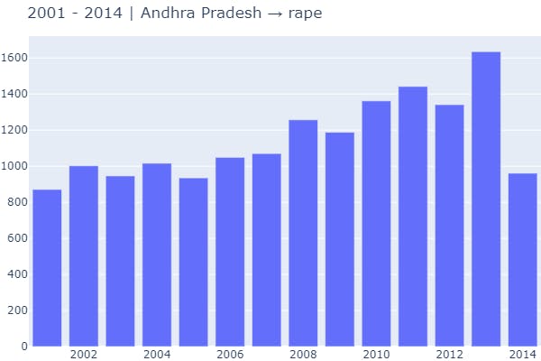
2 Function Call → Visualization of any single crime on the basis of a particular state.

plot_crime_overall_diff(data_source=data_splits, crime='rape', state_unit='Andhra Pradesh')

In the above methods, we considered only the rape column. If we want to identify patterns for any other column, we can do so by changing the parameter value.

---

Plotting the data state-wise and yearly-wise with a specific crime (column) as a target.

1. For this, we will create a function that takes any single crime state-wise or country-wise and at a particular period of time. We just need to provide the data_source, crime, year, and state_unit is optional.

2. If state_unit is specified, it does the same process but only limited to that particular state.

def plot_column(data_source, year, crime, state_unit=None, kind='bar'):
    states_x, crime_y = obtain_features(data_source=data_source, year=year, crime=crime, state_unit=state_unit)

    t = '{} | {} → {}'
    title = t.format(year, crime, state_unit.title()) if state_unit else t.format(year, crime, 'India')

    if kind == 'bar':
        trace = go.Bar(x=states_x, y=crime_y)
    else:
        trace = go.Pie(labels=states_x, values=crime_y)

    layout = go.Layout(
        height=400,
        width=600,
        title=title,
        margin=dict(l=0, r=0, b=0, t=40)
    )

    fig = go.Figure(data=[trace], layout=layout)
    fig.show()

    return None

1 Function Call → Visualization of any single crime on the basis of the whole country in a particular period of time.

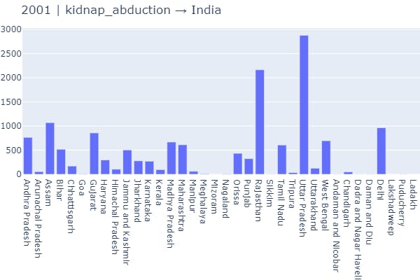
plot_column(data_source=data_splits, year=2001, crime='kidnap_abduction')

2 Function Call → Visualization of any single crime on the basis of a particular state in a particular period of time.

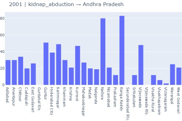
plot_column(data_source=data_splits, year=2001, crime='kidnap_abduction', state_unit='Andhra Pradesh')

Geographical Plot - State-wise Crime Activity

In order to plot the data geographically, we need to have a map layout, and accordingly, the data can be visualized.

Downloading GeoJSON Data - State-wise

def get_india_map(year, state_unit=None):
    if year < 2014:
        if not state_unit:
            return 'https://raw.githubusercontent.com/geohacker/india/master/state/india_state.geojson'
        return 'https://raw.githubusercontent.com/geohacker/india/master/district/india_district.geojson'
    return 'https://raw.githubusercontent.com/geohacker/india/master/state/india_telengana.geojson'

Getting the Districts GeoJSON

def get_districts_json(year, state_unit=None):
    geo_link = get_india_map(year=year, state_unit=state_unit)

    if not state_unit:
        return geo_link

    req_data = requests.get(url=geo_link)
    req_json = req_data.json()['features']

    state_districts = []
    for feature in req_json:
        if feature['properties']['NAME_1'] == state_unit:
            state_districts.append(feature)

    return {
        "type": "FeatureCollection",
        "crs": { "type": "name", "properties": { "name": "urn:ogc:def:crs:OGC:1.3:CRS84" } },
        "features" : state_districts
    }

Visualizing the Choropleth Map

def plot_state_wise(data_source, year, crime, state_unit=None):
    state_unit = None
    state_x, crime_y = obtain_features(data_source=data_source, year=year, crime=crime, state_unit=state_unit)
    df_cols = ['name', 'crime_count']
    state_crime_df = pd.DataFrame(data=zip(state_x, crime_y), columns=df_cols)

    trace = go.Choropleth(
        geojson=get_districts_json(year=year, state_unit=state_unit),
        featureidkey='properties.NAME_1',
        locations=state_crime_df['name'],
        z=state_crime_df['crime_count'],
        colorscale='Reds',
        marker_line_color='black',
        colorbar=dict(
            title={'text': "Crime Range"},
        )
    )

    layout = go.Layout(
        title="{} → Crime Activity - {}".format(year, crime),
        geo=dict(
            visible=False,
            lonaxis={'range': [65, 100]},
            lataxis={'range': [5, 40]}
        ),
        margin=dict(l=0, b=0, t=30, r=0),
        height=600,
        width=600
    )

    fig = go.Figure(data=[trace], layout=layout)
    fig.show()

    return None

1 Function Call - Visualizing dowry_deaths data state-wise based on a particular year.

plot_state_wise(data_source=data_splits, year=2001, crime='dowry_deaths')

plot_state_wise(data_source=data_splits, year=2014, crime='dowry_deaths')

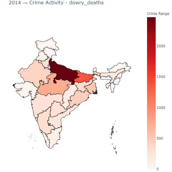
In Uttar Pradesh, we can observe that the count of deaths due to dowry crime was high in both 2001 and 2014.

Observation

1. It is observed that as the count of the year increases there is a drastic increase in the occurrence of crimes. It is quite painstaking to observe this, we are all been told that the development of the country (from every angle) needs time and patience. As the years increase there should be a decrease in occurrences. But it is the opposite.

2. Crimes against women are increasing no matter what measures are taken.

3. Moreover, this dataset includes the activity that had taken place till 2014, we do not know how many more happened to this date.

4. The same pattern is observed when we consider any single state and run our analysis.

---

Well, that's all for now. This article is included in the series Exploratory Data Analysis, where I share tips and tutorials helpful to get started. We will learn step-by-step how to explore and analyze the data. As a pre-condition, knowing the fundamentals of programming would be helpful. The link to this series can be found here.