


Introduction
In this article, we will learn how to add/draw a border to the image. We use OpenCV to read the image. The rest of the part is handled by NumPy to code from scratch. We rely on it for the matrix operations that can be achieved with so much ease.
There are two aspects in which we can start to think:
- If the image is read in grayscale, we can simply keep the default color as black. This is because the length of the shape of the image matrix would be 2. Therefore we cannot add a color border whose color value would be of size 3 and thus it cannot be mapped easily.
- If the image is read in RGB, we can have a choice to pick the color for the border. This is because the length of the shape of the image matrix would be 3. Hence we can add a color border whose color value would be of size 3 which can be mapped easily.
Credits of Cover Image - Photo by Kanan Khasmammadov on Unsplash
Before proceeding further, we need to make sure we have enough colors (based on the user’s choice). I have extracted the possible color values from this website.
The code of the same can be seen below. The result is stored in a JSON file named color_names_data.json.
import requests
import json
from bs4 import BeautifulSoup

def extract_table(url):
    res = requests.get(url=url)
    con = res.text
    soup = BeautifulSoup(con, features='lxml')
    con_table = soup.find('table', attrs={'class' : 'color-list'})
    headings = [th.get_text().lower() for th in con_table.find("tr").find_all("th")]
    table_rows = [headings]
    for row in con_table.find_all("tr")[1:]:
        each_row = [td.get_text().lower() for td in row.find_all("td")]
        table_rows.append(each_row)
    return table_rows

col_url = "https://www.colorhexa.com/color-names"
color_rows_ = extract_table(url=col_url)

color_dict = {}
for co in color_rows_[1:]:
    color_dict[co[0]] = {
        'r' : int(co[2]),
        'g' : int(co[3]),
        'b' : int(co[4]),
        'hex' : co[1]
    }

with open(file='color_names_data.json', mode='w') as col_json:
    json.dump(obj=color_dict, fp=col_json, indent=2)
It is necessary to grab R, G, and B values in order for the mapping after the separation of pixels. We follow split and merge methods using NumPy.
The structure of the color data can be seen below.
{
  "air force blue": {
    "r": 93,
    "g": 138,
    "b": 168,
    "hex": "#5d8aa8"
  },
  "alizarin crimson": {
    "r": 227,
    "g": 38,
    "b": 54,
    "hex": "#e32636"
  },
  "almond": {
    "r": 239,
    "g": 222,
    "b": 205,
    "hex": "#efdecd"
  },
  ...
}
Time to Code
The packages that we mainly use are:
- NumPy
- Matplotlib
- OpenCV
Import the Packages
import numpy as np
import cv2
import json
from matplotlib import pyplot as plt
Read the Image
def read_this(image_file, gray_scale=False):
    image_src = cv2.imread(image_file)
    if gray_scale:
        image_src = cv2.cvtColor(image_src, cv2.COLOR_BGR2GRAY)
    else:
        image_src = cv2.cvtColor(image_src, cv2.COLOR_BGR2RGB)
    return image_src
The above function reads the image either in grayscale or RGB and returns the image matrix.
Code Implementation with Library
For adding/drawing borders around the image, the important arguments can be named as below:
image_file→ Image file location or image name if the image is stored in the same directory.bt→ Border thicknesscolor_name→ By default it takes 0 (black color). Otherwise, any color name can be taken.
We use the method copyMakeBorder() available in the library OpenCV that is used to create a new bordered image with a specified thickness. In the code, we make sure to convert the color name into values from the color data we collected earlier.
The below function works for both RGB image and grayscale image as expected.
def add_border(image_file, bt=5, with_plot=False, gray_scale=False, color_name=0):
    image_src = read_this(image_file=image_file, gray_scale=gray_scale)
    if gray_scale:
        color_name = 0
        value = [color_name for i in range(3)]
    else:
        color_name = str(color_name).strip().lower()

        with open(file='color_names_data.json', mode='r') as col_json:
            color_db = json.load(fp=col_json)

        colors_list = list(color_db.keys())
        if color_name not in colors_list:
            value = [0, 0, 0]
        else:
            value = [color_db[color_name][i] for i in 'rgb']

    image_b = cv2.copyMakeBorder(image_src, bt, bt, bt, bt, cv2.BORDER_CONSTANT, value=value)

    if with_plot:
        cmap_val = None if not gray_scale else 'gray'
        fig, (ax1, ax2) = plt.subplots(nrows=1, ncols=2, figsize=(10, 20))

        ax1.axis("off")
        ax1.title.set_text('Original')

        ax2.axis("off")
        ax2.title.set_text("Bordered")

        ax1.imshow(image_src, cmap=cmap_val)
        ax2.imshow(image_b, cmap=cmap_val)
        return True
    return image_b
Let’s test the above function —
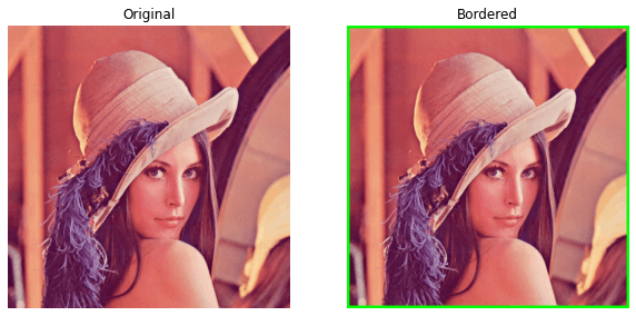
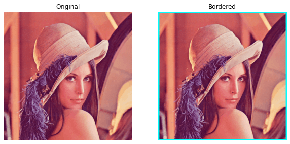
add_border(image_file='lena_original.png', with_plot=True, color_name='green')
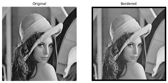
add_border(image_file='lena_original.png', with_plot=True, gray_scale=True, color_name='pink')
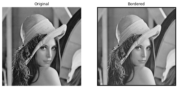
We can clearly see the borders are been added/drawn. For the grayscale image, though we have mentioned pink, a black border is drawn.
Code Implementation from Scratch
When we talk about the border, it is basically a constant pixel value of one color around the entire image. It is important to take note of the thickness of the border to be able to see. Considering the thickness we should append a constant value around the image that matches the thickness level.
In order to do so, we can use the pad() method available in the library NumPy. This method appends a constant value that matches the level of the pad_width argument which is mentioned.
Example
>>> import numpy as np
>>> m = [[1, 2, 3], [4, 5, 6], [7, 8, 9]]
>>> m = np.array(m)
>>> m
array([[1, 2, 3],
       [4, 5, 6],
       [7, 8, 9]])
>>>
>>> pm = np.pad(array=m, pad_width=1, mode='constant', constant_values=12)
>>> pm
array([[12, 12, 12, 12, 12],
       [12,  1,  2,  3, 12],
       [12,  4,  5,  6, 12],
       [12,  7,  8,  9, 12],
       [12, 12, 12, 12, 12]])
>>>
>>> pmm = np.pad(array=m, pad_width=2, mode='constant', constant_values=24)
>>> pmm
array([[24, 24, 24, 24, 24, 24, 24],
       [24, 24, 24, 24, 24, 24, 24],
       [24, 24,  1,  2,  3, 24, 24],
       [24, 24,  4,  5,  6, 24, 24],
       [24, 24,  7,  8,  9, 24, 24],
       [24, 24, 24, 24, 24, 24, 24],
       [24, 24, 24, 24, 24, 24, 24]])
>>>
More examples can be found in the documentation.
We just need to change the constant_values argument by taking the actual color value.
- For a grayscale image, we simply pad the image matrix with black color i.e., 0.
- For the RGB image, we are to grab the color value from the data collected, split the image into 3 matrices, and pad each matrix with each color value. The below function would explain the flow more clearly.
The below function would explain the flow more clearly.
def draw_border(image_file, bt=5, with_plot=False, gray_scale=False, color_name=0):
    image_src = read_this(image_file=image_file, gray_scale=gray_scale)
    if gray_scale:
        color_name = 0
        image_b = np.pad(array=image_src, pad_width=bt, mode='constant', constant_values=color_name)
        cmap_val = 'gray'
    else:
        color_name = str(color_name).strip().lower()

        with open(file='color_names_data.json', mode='r') as col_json:
            color_db = json.load(fp=col_json)

        colors_list = list(color_db.keys())
        if color_name not in colors_list:
            r_cons, g_cons, b_cons = [0, 0, 0]
        else:
            r_cons, g_cons, b_cons = [color_db[color_name][i] for i in 'rgb']

        r_, g_, b_ = image_src[:, :, 0], image_src[:, :, 1], image_src[:, :, 2]
        rb = np.pad(array=r_, pad_width=bt, mode='constant', constant_values=r_cons)
        gb = np.pad(array=g_, pad_width=bt, mode='constant', constant_values=g_cons)
        bb = np.pad(array=b_, pad_width=bt, mode='constant', constant_values=b_cons)

        image_b = np.dstack(tup=(rb, gb, bb))
        cmap_val = None

    if with_plot:
        fig, (ax1, ax2) = plt.subplots(nrows=1, ncols=2, figsize=(10, 20))

        ax1.axis("off")
        ax1.title.set_text('Original')

        ax2.axis("off")
        ax2.title.set_text("Bordered")

        ax1.imshow(image_src, cmap=cmap_val)
        ax2.imshow(image_b, cmap=cmap_val)
        return True
    return image_b
Let’s test the above function —
draw_border(image_file='lena_original.png', with_plot=True, color_name='cyan')
draw_border(image_file='lena_original.png', bt=10, with_plot=True, gray_scale=True)
Yay! We did it. We coded the entire thing including color choice completely from scratch except for the part where we read the image file. We relied mostly on NumPy as it is very fast in computing matrix operations (We could have done it with for loops if we wanted our code to execute very slow).
Personally, this was a great learning for me. I am starting to think about how difficult and fun that would be for the people who actually work on open source libraries.
You should definitely check out my other articles on the same subject in my profile.
If you liked it, you can buy coffee for me from here.